A Thin Rod in a Varying Field: Finding the Maximum Induced EMF ✛
Context
Helmholtz coils produce a nearly uniform field in the open space between them, making them a staple for calibrating magnetometers, in medical cell separators, and in particle detectors. However, beyond the central region the field drops rapidly and even reverses sign, and the behavior of induced EMF in an extended conductor there has been poorly studied. This work presents an experiment with a thin rod that spans the entire radial structure of the field, comparing data with simple models. Neighboring studies in the archive address quantum algorithms and nonlocal magnetic flux transfer, but here the problem is classical and applied: understanding where the induced signal is maximal to better position sensors.
Methods
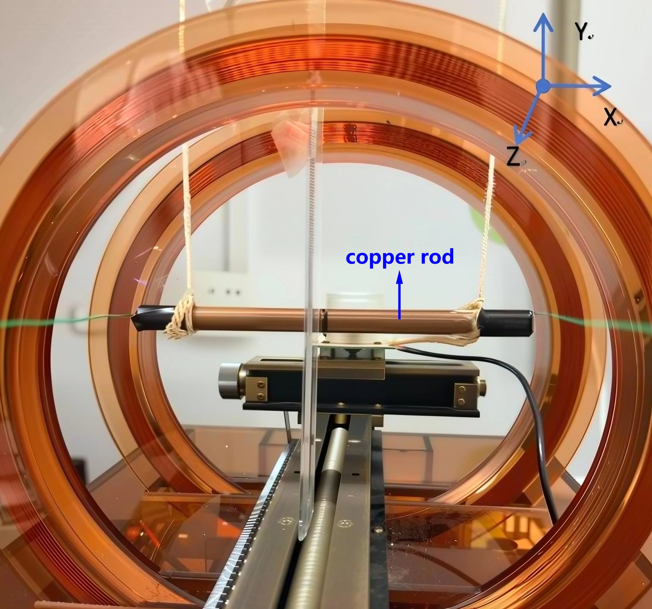
The setup consisted of two coils with a radius of 10.5 cm, 400 turns each, spaced 10.5 cm apart. An alternating current with a frequency of 220 Hz and an effective value of 30 mA was passed through the coils. A copper rod 15 cm long and 1 cm in diameter was placed horizontally in the midplane, with its center moved along the vertical axis in steps of about 1 cm. The induced EMF was measured with a multimeter with an accuracy of 0.001 mV; wires from the rod were routed parallel to the field axis to avoid adding spurious signals. For the theory, four simplified radial field profiles were constructed: a step function (uniform field inside radius R and zero outside), a linear decay, an exponential decay with reverse field, and a piecewise linear fit of six segments. The EMF was computed via the integral of the vortex electric field along the rod, which reduces to the area of a triangle between the center and the rod ends.
Results
The experimental curve shows zero EMF at y=0, reaching a maximum of 0.807 mV at y=9.8 cm (0.933R), then monotonically decaying to 0.285 mV at y=25 cm. All four models give qualitatively the same trend: rise from zero, peak, and decay. Peak positions are: step model at 0.969R (3.84% deviation from experiment), linear at 0.948R (1.59%), exponential at 0.958R (2.65%), and piecewise linear at 0.967R (3.64%). In the central region up to 0.3R, all models match the experiment. In the transition region from 0.5R to 1.26R, the step model underestimates the EMF because it ignores the gradual field decay. Beyond 1.26R, the field reverses sign, and only models with reverse field (exponential and piecewise linear) agree with the data; the piecewise linear model works across the entire range within experimental error.
Implications
This work shows that for an extended conductor, the maximum induced EMF lies not at the coil boundary but slightly inside it, when the central part of the rod is still in the field while the ends have already exited. This is a geometric consequence: the signal is proportional to the area of the triangle traced by the rod and the field center. Compared to neighboring studies focusing on quantum effects or nonlocal transport, here a simple and reproducible method links the shape of the EMF curve to the field profile. The practical value is that sensor calibration can be performed not only in the uniform zone but also at the edge, where the signal is maximal and sensitivity is higher.
Future development
The model can be refined by accounting for the radial field component and the finite rod thickness, which would introduce corrections to the curve shape near the edge. It would be interesting to test the EMF behavior for rods of different lengths: if the length is comparable to the coil radius, the peak might shift or split. For practical purposes, building a sensitivity map for arbitrarily shaped sensors would help optimize their placement in inhomogeneous fields. The approach could also be adapted to three-axis Helmholtz coils, where the field is not axisymmetric.
Impact
The result is directly applicable to magnetometer calibration and the design of induction sensors, where knowing the position of the signal maximum is crucial. The methodology is also useful in teaching laboratories as a vivid demonstration of Faraday's law and the limits of field uniformity in Helmholtz coils.
Next steps
Perform measurements with copper rods of different lengths and diameters to test the universality of the peak position. Compare experimental curves with numerical calculations of the full coil field, including the radial component, and assess its contribution to the EMF.
Key open problems
In classical electrodynamics, the precise treatment of edge effects in inhomogeneous fields for finite-length conductors remains an open question. This work shows that even crude field models suffice for qualitative description, but quantitative agreement requires a detailed profile, including the reverse field. This ties the problem to the broader challenge of calibrating sensors in real, non-idealized fields.
The knowledge machine's view
This section is addressed to the author of the paper and their colleagues. Neighbouring works were found by meaning-based search across our archive, not by word overlap. We do not review: we show the field around the work.
What the work does
The work measured the induced EMF on a thin copper rod moved across the alternating magnetic field of Helmholtz coils. An experimental curve was obtained with a zero at the center, a maximum at y=0.933R, and a monotonic falloff. Four models of the radial field profile were constructed; all qualitatively reproduce the shape of the curve, and the piecewise-linear one gives quantitative agreement over the entire range.
Where its strength is
The strength of the work lies in combining a simple, reproducible experiment with a set of models of varying complexity, which made it possible to identify the key role of the geometric factor, namely the area of the triangle between the center and the ends of the rod, in the position of the EMF maximum.
Where it could go next
- It might be interesting to look at the connection between the geometry of an extended conductor and the topological properties of the field in real space, as was done for electronic bands in the analysis 2412.02813.based on: Where the Electron Lives: Topology of the Band Structure in Real Space arXiv:2412.02813
- Closely related is the approach to turbulent amplification of magnetic fields in neutron stars; perhaps it will suggest how to generalize the models to the case of nonstationary or turbulent fields in calibration setups.based on: Cosmic Kneading: Turbulent Amplification of Magnetic Fields in Newborn Neutron Stars arXiv:2607.21990v1
- The archive contains an analysis of layered crystals that resist rotation; its methods for analyzing edge effects could be useful for refining the behavior of the EMF in the transition zone.based on: A Lid That Twists at Its Rim: How Layered Crystals Resist Rotation arXiv:2609.08931v1
Worth trying
- Check whether the position of the maximum persists when the rod length or the field frequency is changed.
- Use the piecewise-linear model for the inverse problem: reconstructing the field profile from the measured EMF curve.
- Compare the sensitivity of the method with calibration using a point sensor under the same conditions.
Why this may matter
The proposed method of linking the shape of the EMF curve to the field profile could simplify sensor calibration in nonuniform fields and become the basis for educational experiments in electromagnetism.
Nearby works in our archive
- The Deuteron's Electric Dipole Moment: Hunting for Asymmetrysimilarity 0.51
- Cosmic Kneading: Turbulent Amplification of Magnetic Fields in Newborn Neutron Starssimilarity 0.49
- Spy Atoms Catch Weak Signalssimilarity 0.49
- Where the Electron Lives: Topology of the Band Structure in Real Spacesimilarity 0.48
- A Lid That Twists at Its Rim: How Layered Crystals Resist Rotationsimilarity 0.48
- Tantalum Nucleus Reveals Electric Asymmetrysimilarity 0.47
The archive is sparse around this work: the closest review is only 0.51, against a usual 0.64. It looks like few have drilled nearby.
The maximum EMF occurs when the rod is shifted from the center by 93% of the coil radius, meaning its center is almost at the field boundary while its ends are already outside. At this point, the signal is nearly three times larger than at half the radius.
Key numbers
- coil radius: 10.5 cm
- rod length: 15 cm
- current frequency: 220 Hz
- maximum EMF: 0.807 mV
- peak position: 0.933R (9.8 cm)