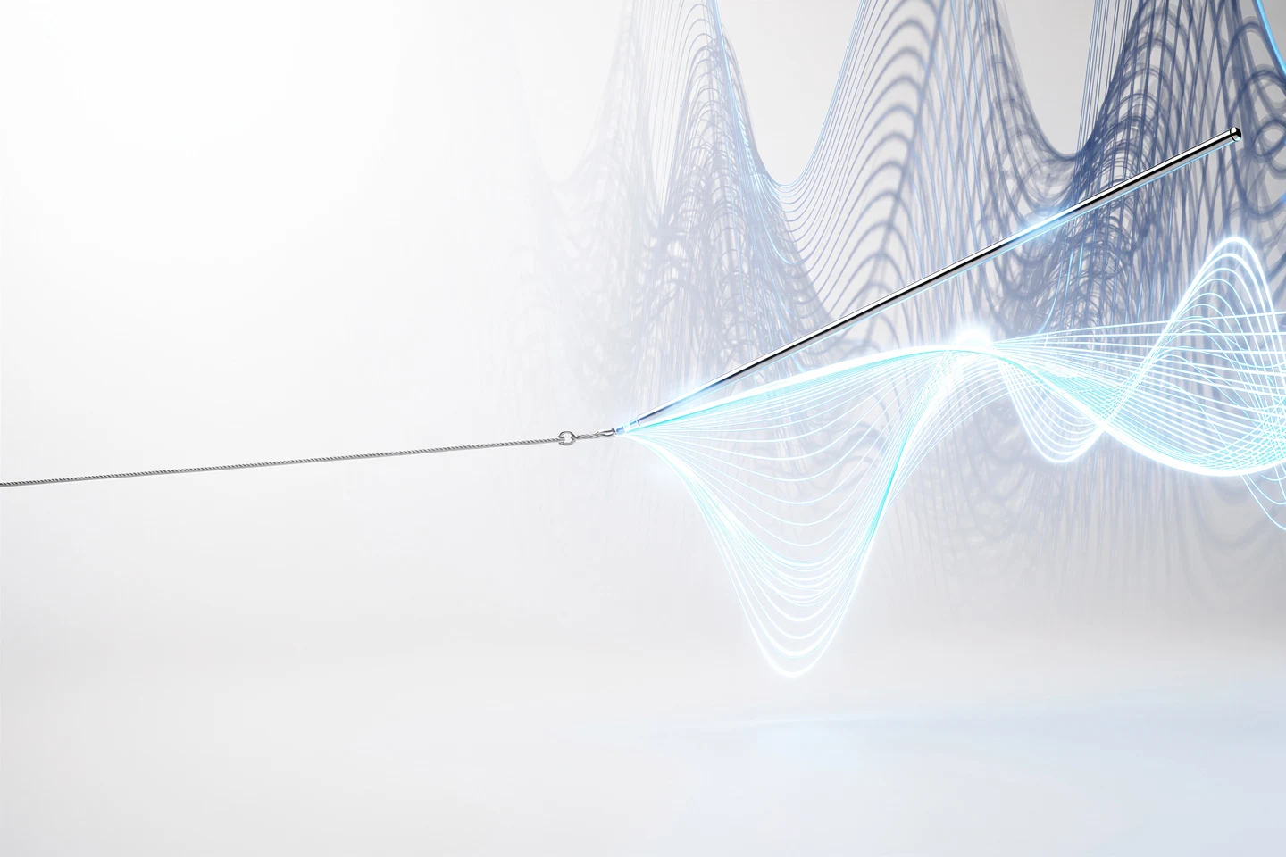
A tightrope walker steps onto the wire. Every move is a calculation: shift your weight just right, or you’ll fall. In the world of quantum particles described by the Dirac equation, there’s a different kind of abyss — the wave function’s furious oscillations. When the scaled Planck constant ε becomes tiny, the solution trembles at a frequency of 1/ε, and tracking its evolution over time directly would require impossibly fine steps in space and time. That’s where operator splitting methods (breaking the evolution into simple pieces) come to the rescue.

The scheme is simple: instead of solving the whole equation at once, you split it into kinetic and potential parts and apply them in turn, just as a tightrope walker shifts weight from one foot to the other. Mathematicians tested three “gaits”: the crude S1 (one kinetic step, then potential), the careful S2, and the elegant S4c. The spatial part is handled by a Fourier spectral method (expanding in trigonometric functions), tracing back to the work of Joseph Fourier, and it delivers near-perfect accuracy.

But how many steps does it take, and what’s the “wobble”? The answer is sharp: the time error for S1 scales like τ/ε², for S2 like τ²/ε³. For graphene, ε ≈ 0.01. To hold accuracy at 10⁻⁶, S1 would need a time step of τ ~ 10⁻⁸ seconds, while S2 manages with τ ~ 10⁻⁵. Ten microseconds — in that time, sound in air travels only 3 millimeters. A thousandfold saving!

These estimates are more than just formulas: they’re a safety line. Knowing how much the method errs lets you boldly enlarge the step and speed up the calculation by orders of magnitude. Simulating electrons in graphene, calculating edge currents in topological insulators from the realm of quantum condensed matter, the creation of electron–positron pairs in ultra-intense laser fields — all of this is now accessible on ordinary computers.

On the horizon are three-dimensional problems and nonlinear versions of the equation, where the kinetic and potential parts no longer split so cleanly. The quantum tightrope walker will need an even more sophisticated gait. But the first step is made: rigorous error bounds turn numerical experiment into a reliable tool, not a guessing game. The tightrope walker no longer balances blind. He knows the limits of his art, and so he steps ever more confidently — deeper into the quantum world.