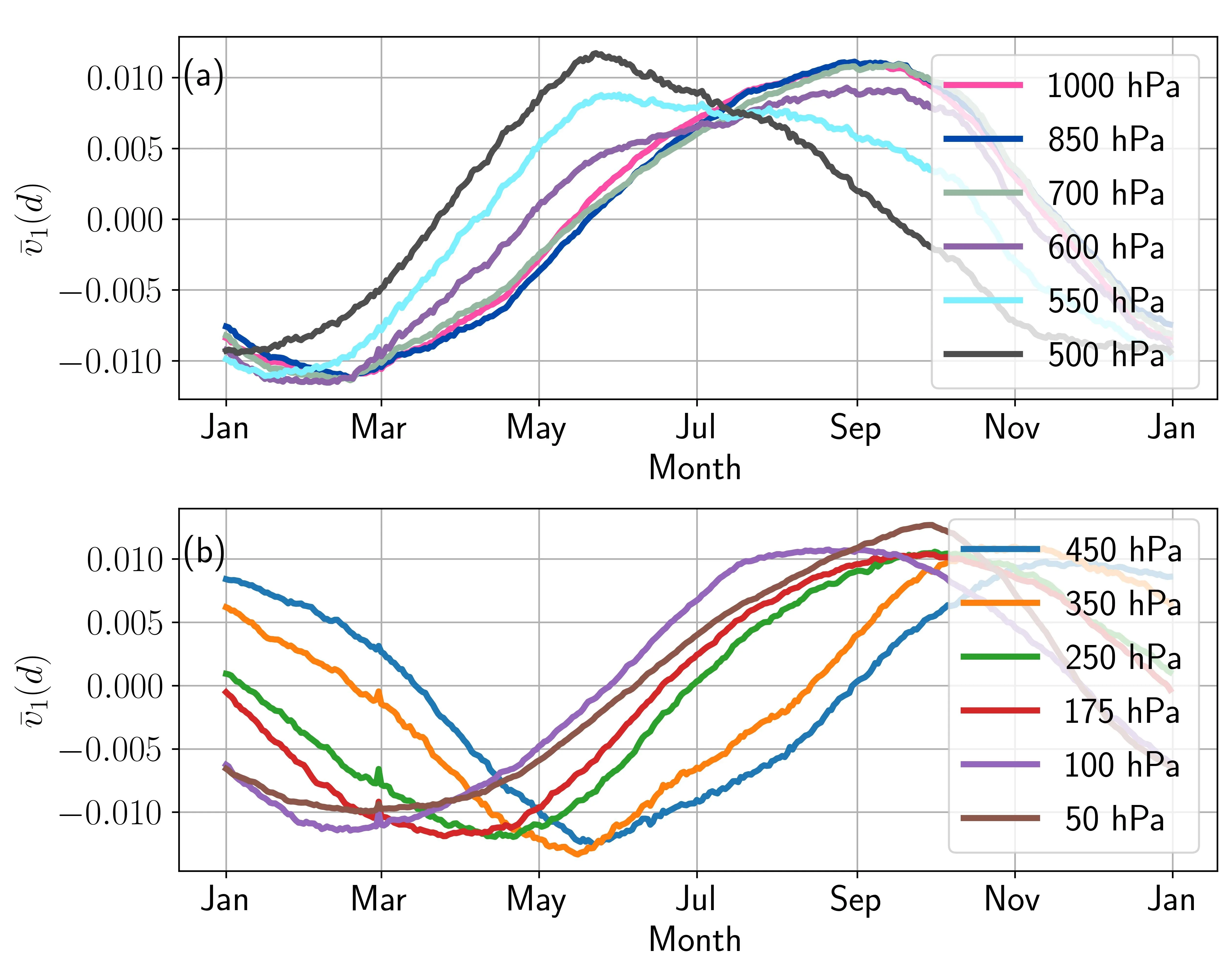
Ozone is like a choir with many voices: near the ground it sings a worrying tune, because it harms lungs and leaves, while at an altitude of twenty-five kilometers it protects us from sunburn. Same gas, but opposite roles. Scientists wanted to understand who is responsible for what in this choir, so they broke it down into individual voices.

They took daily records of ozone concentration in the air over forty-one years, at thirty-seven altitude levels, from the ground to the upper stratosphere. Each point on the map became a singer, and its fluctuations a note. Then they applied a method that automatically finds recurring patterns in these notes, as if extracting clean parts from noise. This revealed different processes: the changing seasons, a long-term trend, the warm El Niño current, stratospheric winds, and the boundary between the lower and upper air layers.

It turned out that each voice sounds louder or softer depending on altitude. For example, the seasonal rhythm is strongest near the ground and in the stratosphere, but fades in between. Meanwhile, the minimum ozone near the surface occurs in February, while at an altitude of twenty kilometers it only arrives in June. So altitude acts like a conductor's baton, controlling the volume of each singer. Now scientists can monitor the ozone layer more precisely and apply this method to other parts of the climate, such as ocean currents.