Ozone's eigenmicrostates: how climate stratifies by altitude
Context
Stratospheric ozone shields us from ultraviolet radiation, while near the surface it harms health and plants. Its variability depends on many processes, from chemical reactions to transport by air currents. Classical methods, such as empirical orthogonal functions, capture only part of the picture because ozone changes simultaneously in the horizontal and vertical. This work sits alongside studies of climate networks and extreme precipitation analysis, where statistical physics helps reveal collective phenomena.
Methods
Daily ozone mass mixing ratios from the ERA5 reanalysis were used, spanning 1 January 1979 to 30 June 2020, on 37 pressure levels from 1000 to 1 hPa, with a horizontal resolution of 2.5° × 2.5°. Each grid point was treated as an agent of the system, and its time series, after normalization, formed a microstate. Singular value decomposition of the ensemble of microstates yielded eigenmicrostates and their evolution. To link modes to physical processes, the LOTUS regression model was applied, which accounts for QBO, El Niño, aerosol optical depth, solar flux, and tropopause height.
Results
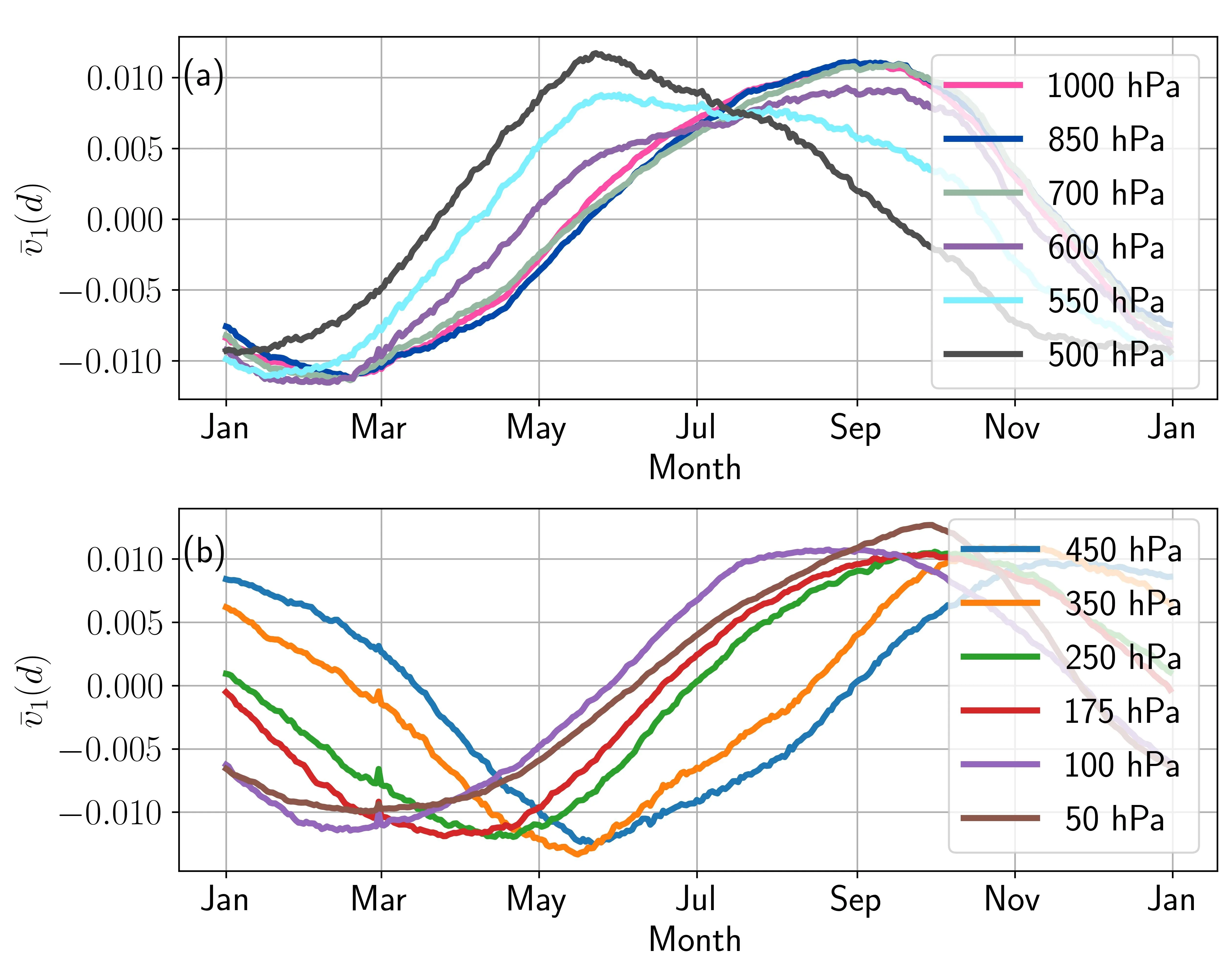
Without removing seasonality, the first eigenmicrostate explains between 10% and 47% of variability depending on altitude: maximum near the surface and in the stratosphere, minimum around 300 hPa. The spatial structure shows two clusters: the Northern and Southern Hemispheres with opposite signs, and the boundary between them shifts northward with altitude. The phase of the annual cycle shifts: the minimum occurs in February near the surface and in June at 50 hPa. After removing seasonality, the first mode reflects the long-term trend, showing ozone decline until the mid-1990s and recovery after 2000 at 50 hPa, which is linked to the Montreal Protocol. The third mode at 100 hPa correlates with tropopause pressure (r = 0.57). El Niño-related modes appear between 400 and 150 hPa, with their correlation to the El Niño index increasing with altitude from 0.24 to 0.47. The quasi-biennial oscillation signal stands out at 50, 30, and 10 hPa with correlations up to 0.67.
Implications
This work shows that the eigenmicrostate method can separate the contributions of different physical processes to ozone variability by altitude. Unlike neighboring studies that focus on individual phenomena or use classical decompositions, here a statistical-physics approach is applied that uncovers collective modes without a priori assumptions. This allows one to see how the same mode changes its spatial structure and significance with altitude.
Future development
The method can be extended to other fields: carbon dioxide distribution, ocean currents. The authors also see potential for detecting tipping points in the climate system, such as the collapse of the Atlantic Meridional Overturning Circulation or Arctic sea ice loss.
Impact
The results are useful for climatology, atmospheric chemistry, and ozone layer monitoring.
Next steps
Apply the method to higher resolution and other variables, such as temperature or greenhouse gas concentrations.
Key open problems
An open question remains about nonlinear interactions between modes and how anthropogenic emissions alter the structure of eigenmicrostates.
The weight of the first ozone mode mirrors the atmospheric temperature profile: both curves have a kink around 300 hPa.
Key numbers
- data period: 1979–2020, 15188 days
- pressure levels: 37 (from 1000 to 1 hPa)
- grid resolution: 2.5° × 2.5°, 10368 points
- maximum QBO correlation: 0.67 at 30 hPa
- first mode weight: from 10% to 47% depending on altitude