Climate as a Conductor: Neural Network Learns to Conduct Extremes ✛
Context
Modeling extreme events in space and time has long been hampered by the rigid assumption of stationarity: the dependence structure between locations was considered fixed. Neighboring papers in the archive show how neural networks learn to recognize patterns in noise or accelerate power system calculations, but almost no one has tried to make a generative model track how the climate regime reshapes the dependence of extremes itself. This work stands apart: its nearest neighbors deal with explainable AI or self-supervised learning, not spatiotemporal distribution tails. The authors fill this niche by introducing a climate index directly into the latent space of a variational autoencoder.
Methods
The authors build a conditional variational autoencoder (cXVAE) in which an encoder transforms a spatial field into latent variables, and a decoder reconstructs it given the climate condition. Unlike previous models, the basis functions linking the latent space to observations are not fixed in advance but are learned together with the network. The climate index (e.g., ENSO) is introduced into the latent representation via a linear mapping and then interleaved with latent variables before being fed into a convolutional decoder. To describe tail dependence, they use a noise process with a log-Laplace distribution, which, as shown in a theorem, preserves the same tail index as the Fréchet distribution. Training is performed on a single CPU without a GPU; for simulations, convergence is reached in about 1000 epochs (about 223 seconds), and for real fire weather data, in 600 epochs (about 981 seconds).
Results
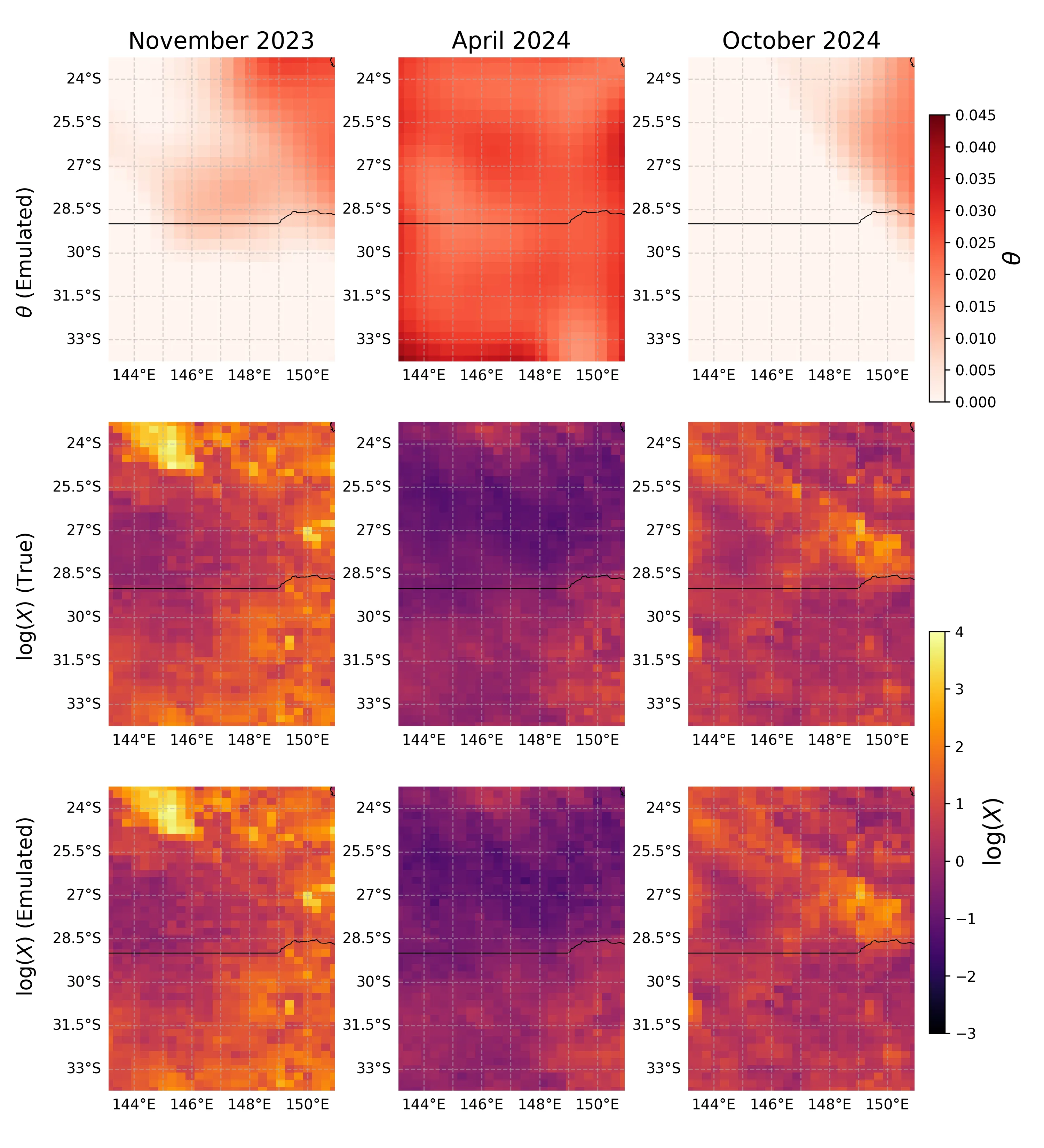
On synthetic data, the model successfully recovers the spatiotemporal structure of the parameter controlling tail heaviness and accurately emulates extreme fields. The extremal dependence coefficient χ between pairs of locations is reproduced with almost no bias at short, medium, and long distances, and the average radius of exceedances (ARE) matches the true value across the entire range of quantiles. The tail-weighted CRPS shows that including a real climate index instead of white noise substantially improves reconstruction quality, and learnable basis functions provide an additional gain. A counterfactual experiment with a flipped ENSO index leads to noticeable shifts in the distributions of emulated extremes, confirming the model's sensitivity to the climate driver. On real data of monthly maxima of the fire weather index in eastern Australia, the model accurately reproduces spatial clustering and tail dependence, with the ENSO influence being moderate, consistent with the known complexity of the link between ocean temperature and fire danger.
Implications
This work shows that deep generative models can replace expensive statistical methods for nonstationary spatiotemporal extremes. Unlike neighboring approaches that either fix the dependence or require huge computational resources, cXVAE trains in minutes on a standard laptop and immediately provides a tool for counterfactual analysis. This is the first demonstration that a climate index can be directly embedded into the latent space of an autoencoder and thereby control tail dependence. The practical value is that the model allows assessing how important a given climate factor is for the joint occurrence of extremes, without running full-scale climate simulations.
Future development
A natural extension involves moving from scalar climate indices to multivariate conditions, for example, spatial fields of sea surface temperature or soil moisture. Another direction is adaptive regularization of temporal smoothness, which is currently applied uniformly, although real systems may undergo abrupt regime shifts. Also promising is teaching the model to handle data on irregular grids and with varying spatial resolution, which would allow combining observations from different sources.
Impact
The method is directly applicable to fire risk assessment, hydrological forecasting, and natural catastrophe insurance, where the joint probability of extremes at multiple locations matters. It is also useful for climate scientists who need a fast way to test how tail dependence would change under a given scenario of climate index change.
Next steps
Immediate next steps include extending the model to multivariate climate conditions and testing on other types of extreme events, such as precipitation or wind speed. It is also worth exploring adaptive temporal regularization schemes so that the model better captures abrupt transitions between climate regimes.
Key open problems
In extreme value statistics, an open question remains how to model nonstationary dependence in high dimensions without losing statistical efficiency. This work directly relates to the problem of identifiability of time-varying tail dependence parameters with limited replication, and to the task of choosing between asymptotic dependence and independence. Furthermore, it touches on the long-standing trade-off between model flexibility and computational feasibility in a spatiotemporal context.
The knowledge machine's view
This section is addressed to the author of the paper and their colleagues. Neighbouring works were found by meaning-based search across our archive, not by word overlap. We do not review: we show the field around the work.
What the work does
The authors build a conditional variational autoencoder (cXVAE) that embeds a climate index into the latent space to model spatiotemporal extremes. The model uses learnable basis functions and log-Laplace noise to preserve tail dependence, and is trained on monthly maxima of the fire weather index in eastern Australia. Results show accurate reproduction of the spatial structure of extremal dependence and sensitivity to the climate driver, with a moderate ENSO influence.
Where its strength is
The strength of the work lies in directly introducing the climate index into the latent space of a variational autoencoder, which allows modeling nonstationary tail dependence without fixed basis functions. This opens the door to fast scenario calculations for fire risk assessment on standard hardware.
Where it could go next
- It might be interesting to see how approaches for separating climate signal from noise, as discussed in the weather-vs-climate paper, could help interpret cXVAE latent variables and improve counterfactual scenarios.based on: Weather vs. Climate: How to Tell Noise from Signal arXiv:2608.14455v1
- Related work on climate giving an early signal suggests considering precursors or early indicators as conditioning inputs to enhance the model's predictive power.based on: When Climate Sends an Early Signal arXiv:2607.11935
- Ideas from the paper on the fourth spring of climate could suggest ways to incorporate additional climate modes or nonlinear interactions into the conditional part of the model.based on: The Fourth Spring of Climate arXiv:2602.10369
Worth trying
- Try conditioning not only on the current ENSO index but also on its lagged values or derivatives to capture delayed effects.
- Use latent space interpretation methods, such as visualizing latent trajectories for different climate regimes, to better understand how the model encodes nonstationarity.
- Test the model's transferability across regions by training on eastern Australia and testing on other fire-prone areas with similar data.
Why this may matter
This approach could become the backbone for operational assessment of climate-driven risks of extreme events, enabling rapid scenario generation under different climate conditions without expensive climate models.
Nearby works in our archive
- Radar Sculptor: How Radio Waves Sculpt a Drone's Portraitsimilarity 0.49
- Ultraviolet Trap: How TRAPPIST-1 Star Fakes Signs of Lifesimilarity 0.48
- The Fourth Spring of Climatesimilarity 0.48
- How the Brain Learns to Look Aheadsimilarity 0.47
- A neural network tastes the atmospheres of distant planetssimilarity 0.47
- When Climate Sends an Early Signalsimilarity 0.47
- Weather vs. Climate: How to Tell Noise from Signalsimilarity 0.46
The archive is sparse around this work: the closest review is only 0.49, against a usual 0.64. It looks like few have drilled nearby.
Training the model on 127 monthly maxima of the fire weather index took about 16 minutes on a standard desktop computer without a graphics accelerator, whereas classical Bayesian methods for similar problems may require many hours or even days.
The idea of 'what if the climate were different' echoes Kim Stanley Robinson's novel 'The Ministry for the Future', where climate scenarios are used to plan disaster prevention. Only here, instead of global models, there is a fast neural network that produces plausible extreme fields in seconds under a modified El Niño index.
Key numbers
- training time on simulations: 223 seconds (about 1000 epochs)
- training time on real FWI data: 981 seconds (about 600 epochs)
- number of locations in FWI data: 1118 points on a 0.3125°×0.25° grid
- FWI data period: May 2014 – November 2024 (127 monthly maxima)
- number of latent nodes in simulation: 64 (8×8 grid)