The Spacetime El Niño Oscillator
Context
El Niño has been studied for decades, but its spatial diversity and temporal irregularity remain a challenge. Alongside this work in the archive are studies that either predict El Niño a year and a half in advance or explore oscillations in other systems, such as neutron stars or galaxy distributions. This article stands apart: it neither predicts nor measures, but builds a theoretical framework that unifies spatial and temporal aspects into a single picture. It is an attempt to answer the question posed in a recent review: can we achieve a conceptual understanding of El Niño diversity in the same way that the simple recharge oscillator model did for the basic dynamics?
Methods
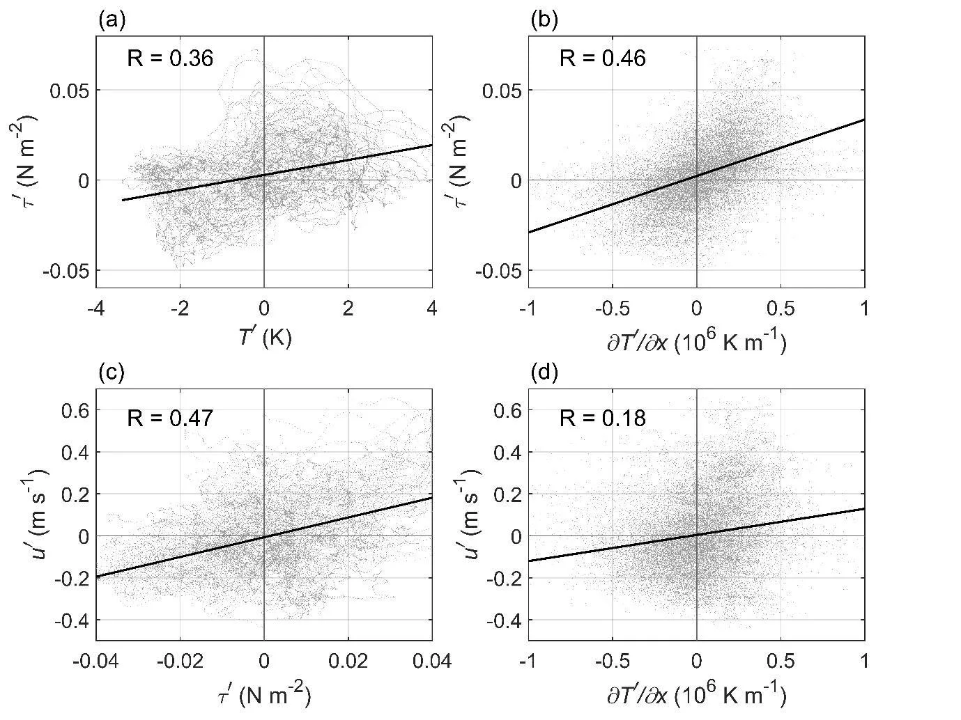
The author starts with the temperature equation for the upper mixed layer of the ocean and the equation for the thermocline depth anomaly. The key step is replacing the zonal current anomaly with the gradient of the sea surface temperature anomaly. This is based on the observation that wind stress, and consequently the current, are proportional not to the anomaly itself but to its spatial gradient. This relationship closes the system and turns it into a wave equation. The solution is sought by expanding in cosines, yielding a set of spatial modes, each oscillating at its own natural frequency. Model parameters, including the coupling coefficient, are estimated from SODA reanalysis data version 3.4.2.
Results
The first spatial mode describes the temperature contrast between the eastern and western Pacific and oscillates with a period of about 4.3 years, corresponding to the eastern Pacific El Niño and the quasi-quadrennial mode. The second mode highlights the contrast between the center and the edges of the basin, oscillates with a period of 2.3 years, and reproduces the central Pacific type. Combining the first two modes with different weights yields complex spatial patterns: for example, strengthening the first mode leads to strong events like the El Niños of 1982/83, 1997/98, and 2015/16. External heating adds forced frequencies, further complicating the time series. The model also predicts wave propagation eastward and westward at speeds consistent with observations.
Implications
Unlike neighboring works that focus on prediction or observation, this article provides an analytical framework linking spatial patterns to temporal periods. It shows that the two types of El Niño are not independent phenomena but arise as different combinations of the same fundamental modes. This changes the view of El Niño diversity: instead of classifying events by type, one can describe them as superpositions of modes with different weights. Such an approach opens the way to a more systematic understanding of complex variability.
Future development
The model can be extended by adding nonlinear terms, stochastic forcing, and the seasonal cycle. This would allow exploring the asymmetry between El Niño and La Niña, phase synchronization, and amplitude modulation. One could also refine the relationship between current and temperature gradient by including an additional term proportional to the anomaly itself, which would improve agreement with data. Further development could lead to a tool for analyzing and predicting specific events.
Impact
The results may be useful for climatologists studying natural variability of the tropical Pacific and for seasonal forecasting specialists, as the model provides a physical basis for interpreting spatial patterns.
Next steps
The next step could be incorporating nonlinearity and stochastic forcing into the model, as well as testing predictions on longer observational records.
Key open problems
This work directly addresses the unresolved problem of explaining the diversity of El Niño spatial patterns and its temporal irregularity. It offers a unified framework that may help understand why events differ in strength, location, and duration.
The period of the second mode is exactly half that of the first, reminiscent of overtones in music: the fundamental tone and its octave create a complex melody of climate oscillations.
Key numbers
- Period of the first mode: 4.3 years
- Period of the second mode: 2.3 years
- Wave propagation speed: 0.25 m/s
- Basin width: about 15000 km
- Coupling coefficient: 1.25·10-5 m²/(s·K)