Multi-Day Rainstorms: How Dynamics Teaches Statistics to Keep Its Story Straight ✛

‹›

In February 2022, the eastern coast of Australia was hit by rains that lasted several days in a row. Water inundated towns in Queensland and New South Wales, insurers paid out 3.35 billion dollars, and the flood became the costliest in the country's history. Meteorologists have long known how to estimate the probability of a single very rainy day, but when a downpour stretches over two or three days, the usual calculations start to lie. Statistics looks at each day in isolation and fails to notice that rainy days come in chains, like cars of a train.

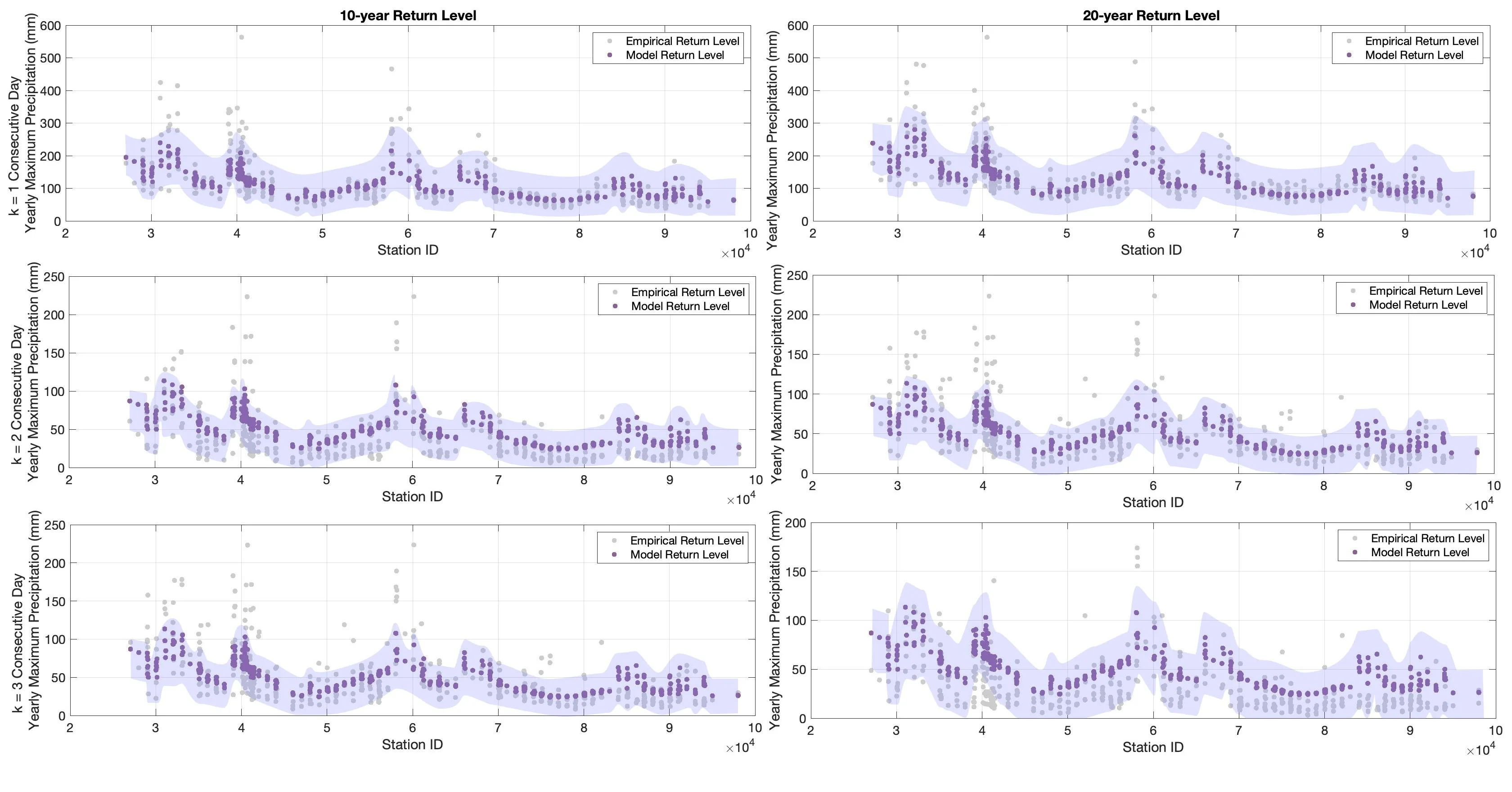
The authors of the new study decided to borrow from dynamical systems the ability to see the whole chain. They took daily rainfall records from 454 weather stations in eastern Australia for 1984–2021 and, for each station, constructed a running minimum over a window of several days. If the window is three days long, then for each day they take the weakest rain among that day and the two following. This trick couples the days: if rain falls on consecutive days, the window minimum stays high, but if the rain is isolated, the minimum drops. They then applied standard extreme-value statistics to these minima, but with one important correction.

The correction came from a recent theorem on max-stability. It says that the shape of the distribution of maxima should not change when we enlarge the window. In practice, this acts as an honesty check: if the shape starts to drift, a numerical error has crept into the calculations. The authors computed that for a three-day window, the relative error in shape is 52.26%, which is still acceptable, but beyond that the data become too sparse. This check is invisible to standard methods and prevents mistaking an artifact for a physical pattern.

The model also accounted for the fact that eastern Australia's climate is not uniform. It included the Southern Oscillation Index (a measure of El Niño or La Niña phase), distance from the coast, latitude, and longitude. The results show that El Niño's influence on three-day extremes is twice as strong as on one-day extremes, and is especially pronounced inland. For example, at the Karange Model Farm station, the probability of a three-day extreme increases by 4.3% when shifting from El Niño to La Niña, whereas on the coast the increase is only 1–1.5%.

So statistics, which used to break the chain of rainy days, has learned to see it whole. The method can be transferred to other regions where rainfall maxima follow the same law, and even to heatwaves. For cities, farms, and insurance companies, this means more accurate risk assessments: not just “someday there will be a heavy downpour,” but “how many days in a row it might last, and with what probability.”