El Niño: Randomness with an Annual Rhythm
Context
A tradition has already formed around this work: some models capture El Niño's rhythm through seasonal cycles, others recover hidden variables from sparse data, and still others explore how random kicks generate large events. Neighboring works on gravitational waves and large-scale structure also rely on stochastic modeling and Gaussian processes, but here the object is different: a climate oscillation with a pronounced annual periodicity. The paper stands apart: its nearest neighbors are far in meaning, which is rather a plus, because the problem demands its own toolkit.
Methods
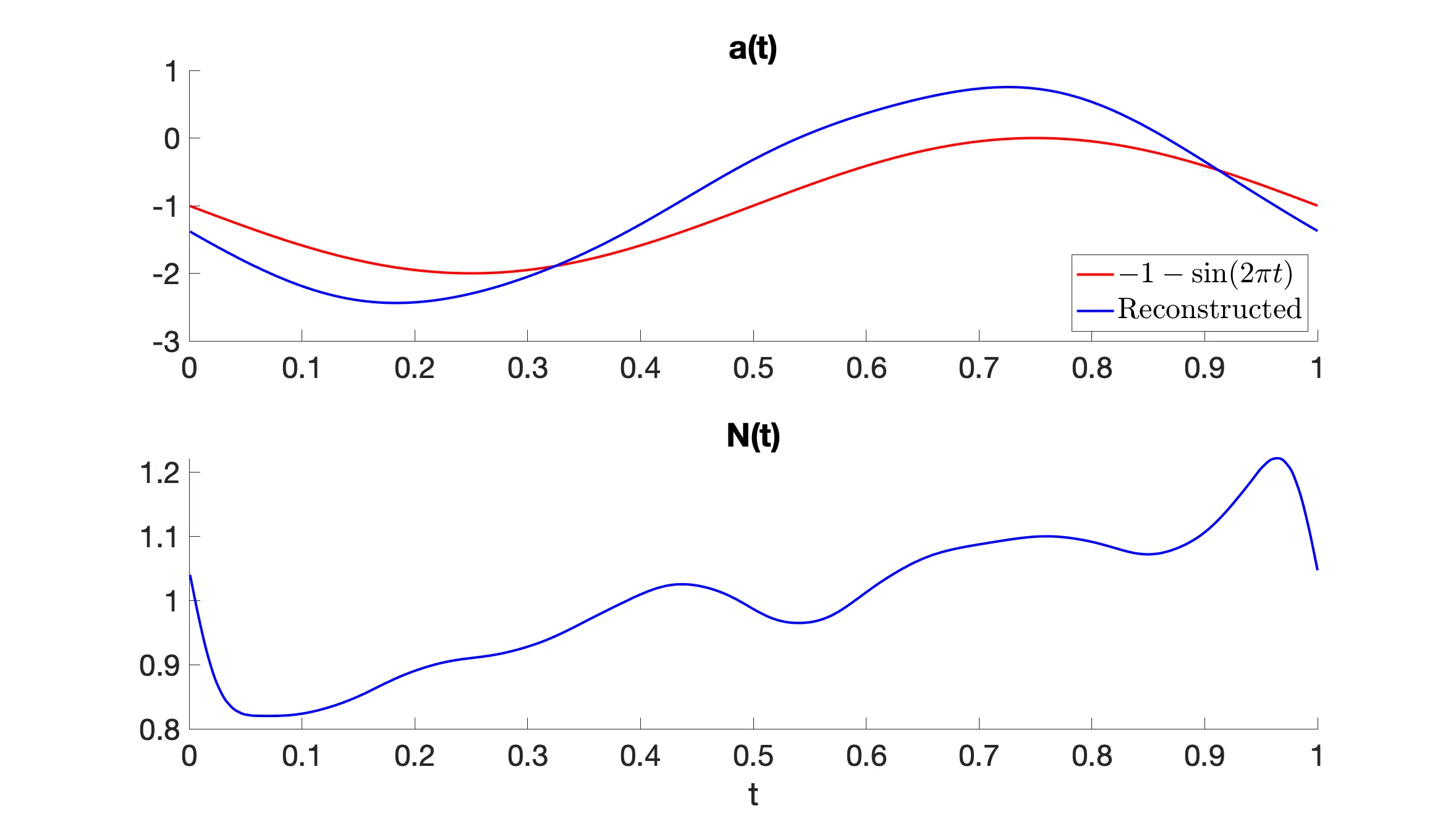
The model starts with two equations for sea surface temperature in the Niño 3.4 region and thermocline depth. The coefficients a(t) and N(t) are estimated directly from monthly statistics of the Niño 3.4 index, while ω(t), λ, and σ are tuned by an expectation-maximization algorithm that handles incomplete data. Then a third equation for wind bursts with multiplicative noise is added to the system. To recover the hidden variables, the conditionally Gaussian structure is exploited: given the ocean temperature, the thermocline and wind bursts remain Gaussian processes, which yields closed-form formulas for the filter and smoother.
Results
The model reproduces the monthly standard deviations of the Niño 3.4 index with high accuracy, and the autocorrelation function matches observations up to three years. Phase locking to the end of the calendar year is visible as a maximum of the standard deviation in November–December. The spring predictability barrier arises from the growth of the noise amplitude N(t) in spring. After adding wind bursts, the temperature distribution becomes non-Gaussian: the model captures the asymmetry and heavy tails. The recovered thermocline depth correlates with observations at 0.9, and the error lies within one standard deviation of the filter.
Implications
Unlike neighboring works, which either recover statistics or predict individual events, this one combines two steps: estimating seasonal coefficients and simultaneously recovering hidden variables. This is the first test of whether multiplicative noise in wind bursts can be introduced into a low-dimensional model without losing analytical tractability. Such a hybrid of physics and statistics yields higher accuracy than global climate models at negligible computational cost.
Future development
The approach can be transferred to other climate oscillations with seasonal locking, such as monsoons or the Arctic Oscillation. Long sea surface temperature records since 1870 allow recovering the thermocline and wind bursts over a century and a half, opening the way to validating climate reconstructions from proxy data. Extension to multivariate indices, such as the zonal temperature gradient, could improve forecasts up to a season ahead.
Impact
Improved seasonal forecasts of El Niño will affect agriculture, water resource management, and insurance in tropical regions. The recovered wind burst series may be useful for calibrating parameterizations in global climate models.
Next steps
Test the model on independent data after 2016 and compare with forecasts from operational centers. Include the zonal temperature gradient to distinguish eastern and central El Niño types.
Key open problems
For climate dynamics, the question remains open why some El Niños become extreme while others decay. The work shows that the key lies in the nonlinear interaction of the seasonal cycle and random wind bursts, but the mechanism selecting extreme events has yet to be understood.
Wind bursts in the western Pacific last only a few days, but their cumulative effect is comparable to the energy of an entire season.
Key numbers
- correlation of recovered thermocline with observations: 0.9
- period of ocean temperature data: 1870–2016
- period of thermocline and wind burst data: 1983–2016
- decay time of wind bursts: 0.25 year
- amplitude of seasonal feedback cycle: 1.5