autocorrelation function

The orchestra plays without a conductor. Each instrument follows its own schedule: the violin on Monday, the flute on Wednesday, the timpani on Saturday. Astronomers hear not music but isolated notes scattered across the calendar. A telescope sees a star only when it is above the horizon and when the schedule has allotted time for it.

An old water pipe hums differently from a new one. A pipe that has lost its flexibility answers every surge of water with a sharp echo that races back to the pump faster than in a young system. Something similar happens with our arteries: over the years their walls harden, and the pulse wave, having reached the small vessels, reflects back to the heart almost without delay.

A doctor places a stethoscope on the chest and listens: lub-dub, lub-dub. The rhythm is there, but how do you measure it when it's noisy around and the patient can't lie still? Conventional devices look for sharp peaks in the heartbeat recording, like catching hammer blows. But if the hammer hits a pillow instead of an anvil, the peaks blur and the device gets lost. CORAL, the new method, works differently.

The quantum world does not forgive forgetfulness. Throw a stone into a pond — the ripples spread and vanish, the information about the impact dissipates without a trace. In quantum mechanics, everything is different: the evolution of a system is reversible, and the past is never completely erased.

A weather forecaster draws a thick black line across Europe: north of it, frost; south, a thaw. That boundary, the zero isotherm, won't tell you the temperature in Stockholm or Rome, but it honestly marks where winter ends. In recent cosmology, a map has emerged where a similar frontier can be drawn.

Every month, satellites measure temperature and humidity over different parts of the planet. Over 24 years, thousands of such paired measurements have accumulated. Normally, temperature and humidity change in concert: when it warms, the air holds more water; when it cools, it releases it. But before a sharp climate shift, this coordination breaks down.

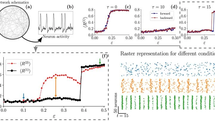
A neuron sends a signal to its neighbor. The neighbor doesn't respond immediately — the impulse travels along the process at a finite speed, like a letter delayed in transit. Usually, such a delay is considered a nuisance, but in this new work, it becomes the conductor. When two excitable neurons are connected with a delay, a rhythm spontaneously emerges between them.

A dance of hundreds of particles: some pairs spin slowly and gracefully, others twitch in a frantic rhythm. To understand the essence of the dance, you need to watch the slow movements: they are the main choreography of the system. In molecular science, such slow movements are called 'slow modes,' and they determine how a protein folds into a ball or how a drug binds to its target.

When the conductor leaves the orchestra, the musicians keep playing from memory for a while. But without a unified rhythm, each one starts to speed up or slow down on their own, and the harmonious symphony turns into disjointed noise. According to new research, the brain and heart behave much the same way in the last hours of a person's life.

A charged particle streaks through a silicon sensor, leaving behind a trail of free electrons. The time it takes for this charge to be collected at the electrode depends on how deep in the crystal it was born. A particle entering head-on carves identical paths through neighboring pixels: their signals arrive almost simultaneously.

A melody plays, and the brain doesn't just listen note by note. It works like a conductor who already knows the score: each next note is expected because the previous ones still echo in memory. But how do neurons hold on to that echo?

The quantum world does not like being pinned down to exact numbers. Physicists usually expand a complex interaction into a long series, like a sum of ever-smaller corrections.

When a person breathes, air doesn't flow in a steady stream but in waves. Previously, doctors and scientists only looked at overall numbers: how much air entered per breath, what the peak flow was. But within a single breath, there are nuances — small variations that speak to the workings of nerves and muscles. The new approach breaks a breath into parts, much like a musician breaks a chord into individual notes.

Each breath slightly speeds up the heart, and each exhale slows it down. This rhythm, visible on an ECG, is called respiratory sinus arrhythmia. For a long time, it was dismissed as a mere side effect of the nervous system. But new research shows that this coordination is not a coincidence: it's a way to save energy.

A piece of aluminum alloy is heated, and it quietly tells you about its strength. You just need to listen to that story in how the metal absorbs heat. The usual way to find out how strong an alloy is — pull it until it breaks. That takes time and destroys the sample.

Two clocks in different rooms need to tick in unison. Usually, this is done by sending bright pulses or pairs of photons that arrive one right after the other. But the signal can be so weak that photons barely make it through. In this work, clocks were synchronized with light a billion times dimmer than usual.

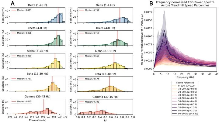
A rat runs down a track — not because a motor forces it, but because it feels like it. On its skull sits a grid of 32 tiny sensors, like a swim cap with wires. The sensors pick up the faint electrical waves emitted by the brain. Previously, to find out how fast an animal was running, you had to implant electrodes directly into the brain.

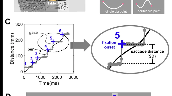
When the hand draws a line, the gaze almost always runs ahead, like a scout peeking around the corner before the column turns. But how far ahead? It turns out that each person has their own distance, and it does not change from attempt to attempt. In the experiment, professional calligraphers and ordinary people traced a contour on a screen while instruments recorded eye and pen movements.

Time flows slower near the ground than on the roof: this was predicted by Einstein in his theory of relativity. To spot the tiny difference, physicists propose using a pair of photons, linked like voices in a duet.

Strike a gong and the sound fades in layers: the low hum lingers longer, the high overtones vanish first, leaving silence behind. So too a qubit, living its quantum life, leaves not one but three echoes of its own past.

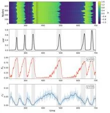
A fisherman pulls on his net and listens to it ring. Each strand quivers in its own way, but before a strong tug, all the strands begin to vibrate in unison. So it is with complex systems: before a sharp state jump, the individual parts suddenly start to oscillate in concert, and that synchrony betrays the coming jump.

In a tropical forest, the dry season gives way to the rainy season, and with the weather, the rules of life change: some animals go into hibernation, while others come out of hiding. Likewise, in complex systems, from climate to economics, the links between processes are not set in stone. They depend on a hidden "regime" that itself switches from time to time.