Points of No Return in El Niño: How Delay Breeds Climate Chaos ✛
The Pacific Ocean remembers. Water warmed off the coast of Peru drifts slowly westward, and six months later its heat returns to South America. Scientists call this six-month journey the delay. It turns a simple climate model into a maze where the route depends not only on your current position but also on where you were half a year ago.
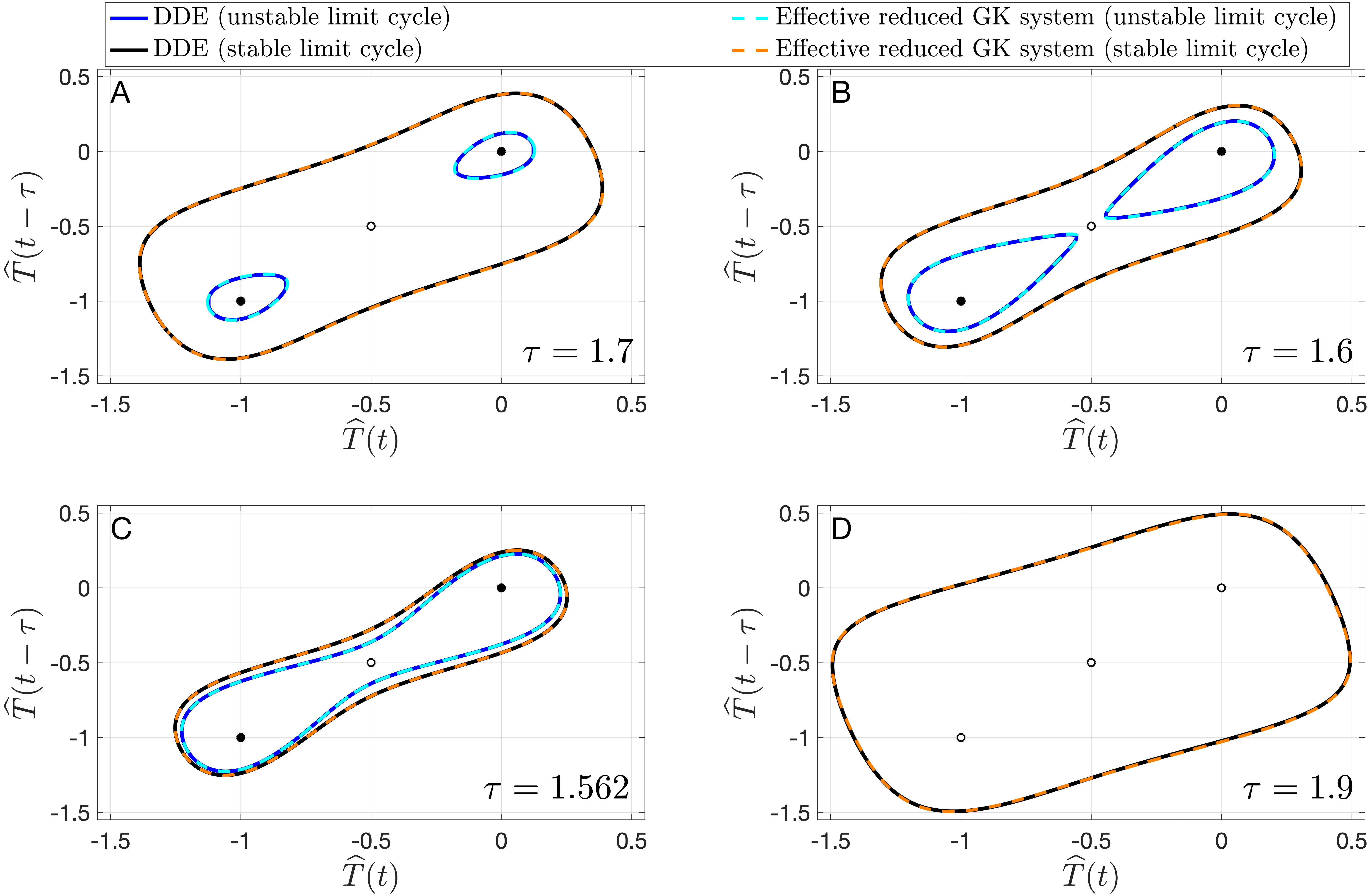
When the delay changes, the maze reshapes itself. At a delay of about 1.74 years, the system loses its stable equilibrium and begins to oscillate. But the oscillations do not become chaotic right away. First, an unstable periodic orbit is born: a closed trajectory that the system repels. If a random kick pushes the state aside, it may wander for a long time before returning.
The authors reduced the complex equation to a two-dimensional system and found three key points: the onset of oscillations, the appearance of a loop connecting an unstable state to itself, and the disappearance of stable cycles. These points, like invisible landmarks, define the boundaries of possible routes.
Then noise was added to the model. Random disturbances, like gusts of wind, constantly knock the system off course. Meanwhile, a slow drift of the delay, mimicking changes in wave travel time, makes the maze slowly change shape. As a result, episodes resembling real El Niño and La Niña appear: warm phases give way to cold ones, and the rhythm is irregular.
Spectral analysis revealed two peaks: around 5.5 years for interannual variability and around 21 years for decadal variability. The decadal peak is linked to unstable periodic orbits near the homoclinic loop. Wandering through the maze, the system occasionally approaches these orbits and lingers near them for several cycles before being repelled again.
The maze of invisible orbits explains why El Niño is so hard to predict. Even knowing all the bifurcations, we cannot say exactly where the system will turn next. But understanding which routes are possible helps us recognize when we are approaching a point of no return. This could form the basis for early warnings of strong events, and for more accurate climate models that account not only for the current state but also for the ocean's memory.
The Suárez–Schopf model was proposed in 1988 and has since served as a testing ground for studying El Niño. Despite its simplicity, it reproduces key features of the phenomenon, including irregularity and decadal modulations.
The idea that small random perturbations can switch a system between qualitatively different regimes echoes the concept of 'bifurcation points' in science fiction, for instance, in Isaac Asimov's novel 'The End of Eternity', where small changes in the past lead to unpredictable consequences in the future.