Tipping Points in El Niño: How Delay Breeds Climatic Chaos ✛
Context
In climate models, the delay reflects the time it takes for waves to cross the Pacific Ocean. For El Niño, this is about half a year. Delay differential equations are infinite-dimensional, making their analysis challenging. Recent work on approximating such equations with systems of ordinary differential equations has opened the way to detailed bifurcation studies. This work follows that line but goes further: it not only finds bifurcations but shows how they organize stochastic variability, including decadal cycles.
Methods
The authors apply the Galerkin method with a Koornwinder basis to reduce the delay equation to a finite-dimensional system. They then use a center-unstable manifold reduction to obtain a two-dimensional system. For this system, they compute the Lyapunov coefficient that determines the type of Hopf bifurcation and construct a bifurcation diagram via backward integration. Afterward, they add multiplicative noise and a slow drift in the delay parameter, mimicking changes in wave transit time.
Results
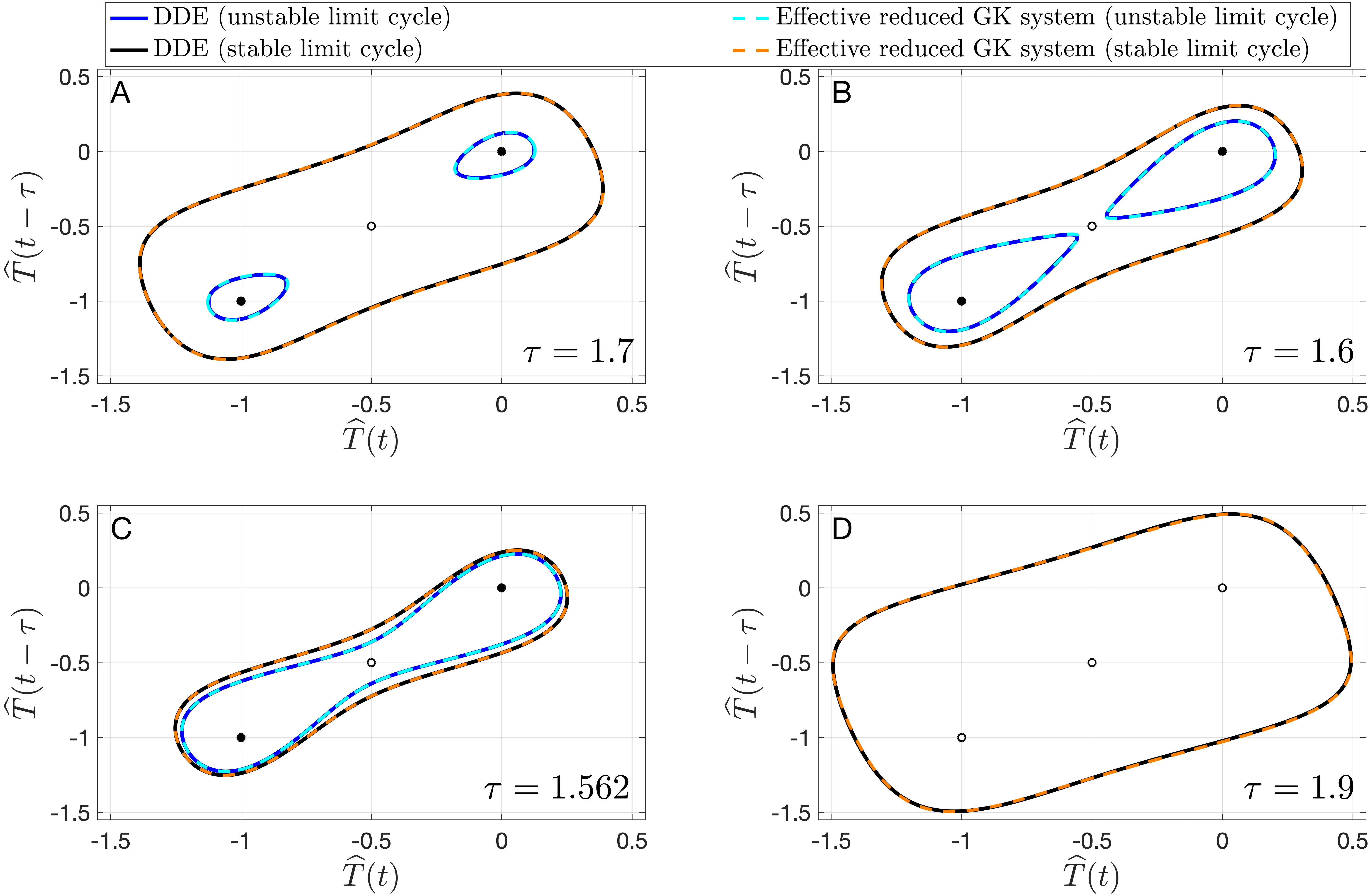
For the Suárez–Schopf model with α=0.75, they find: a subcritical Hopf bifurcation at $τ_c$≈1.7408, a homoclinic bifurcation at τ_♯≈1.5906, and a saddle-node bifurcation of periodic orbits at τ*≈1.5592. The two-dimensional reduced system reproduces these bifurcations with high accuracy, including unstable periodic orbits. The stochastic model with τ drifting from 1.45 to 1.65 produces episodes reminiscent of El Niño and La Niña events. Spectral analysis reveals two peaks: an interannual one around 5.5 years and a decadal one around 21 years. The decadal variability is linked to unstable periodic orbits near the homoclinic loop, for instance, an orbit with a period of 18.23 years.
Implications
This work stands out from neighboring studies because it does not stop at bifurcation analysis but uses it to explain stochastic variability. It shows that transitional paths between invariant sets of the deterministic system, not just equilibria, can organize complex climate patterns. This broadens our understanding of the mechanisms behind El Niño's irregularity.
Future development
The approach can be applied to more realistic models, such as the Cane–Zebiak model, and to models with distributed delays. Exploring the role of the annual cycle and its interaction with unstable periodic orbits is promising. More general parameterizations of the discarded modes could also be used to describe complex bifurcations.
Impact
The results may help interpret observed decadal El Niño variability and aid in developing early warning methods for events.
Next steps
Test the proposed mechanism on models with fuller physics and on observational data. Investigate the influence of the annual cycle on the interaction between noise and unstable orbits.
Key open problems
This work addresses a fundamental problem in climate dynamics: how deterministic bifurcations and noise jointly produce observed irregularity. It offers a concrete mechanism for decadal variability that had not been explicitly linked to homoclinic orbits in delay models before.
The knowledge machine's view
This section is addressed to the author of the paper and their colleagues. Neighbouring works were found by meaning-based search across our archive, not by word overlap. We do not review: we show the field around the work.
What the work does
This study examines the Suarez–Schopf model for El Niño with a time delay. The authors construct a two-dimensional approximation of the original infinite-dimensional system, identify key bifurcations (subcritical Hopf, homoclinic, and saddle-node for periodic orbits), and then add noise and a slow drift in the delay parameter. The resulting trajectories exhibit episodes resembling El Niño and La Niña, and spectral analysis reveals interannual (about 5.5 years) and decadal (about 21 years) peaks associated with unstable periodic orbits near the homoclinic loop.
Where its strength is
The work goes beyond bifurcation analysis by showing how unstable invariant sets of the deterministic system (in particular, unstable periodic orbits) organize stochastic variability, including decadal cycles. This provides a concrete mechanism for complex climate patterns, going beyond simple noise around an equilibrium.
Where it could go next
- It might be interesting to compare the obtained decadal modes with those arising in a seasonally forced model, where resonant phenomena also generate low-frequency variability.based on: How the Seasonal Rhythm Pulls the Strings of El Niño arXiv:2607.00386
- A related work uses chaotic dynamics in a delay model to explain El Niño irregularity; perhaps the stochastic approach in your study could complement deterministic chaos as a source of irregularity.based on: Hidden Rhythms of El Niño: Chaos in the Delay arXiv:2102.11711
- The idea that transition paths between invariant sets organize variability resonates with the concept of 'road maps' of bifurcations; one could consider how your bifurcation structures relate to the global bifurcation picture in coupled models.based on: Climate as a Road Map: Bifurcations and Resonances of El Niño arXiv:1109.2818
Worth trying
- Test whether the decadal peak persists when using realistic noise estimated from observational data instead of parameterized multiplicative noise.
- Investigate the sensitivity of the decadal mode to the shape of the slow drift in the delay parameter (for example, compare linear drift with periodic drift).
- Apply the reduction method to the center-unstable manifold to other delay models (for instance, with two delays) to test the universality of the found bifurcation scenarios.
Why this may matter
If decadal variability is indeed linked to unstable periodic orbits near the homoclinic loop, this could offer a new predictive indicator for long-lasting climate anomalies and aid in interpreting paleoclimate records.
Nearby works in our archive
- Hidden Rhythms of El Niño: Chaos in the Delaysimilarity 0.62
- How the Seasonal Rhythm Pulls the Strings of El Niñosimilarity 0.59
- Climate as a Road Map: Bifurcations and Resonances of El Niñosimilarity 0.58
- Ocean Memory Quenches El Niño Chaossimilarity 0.57
- Three Rhythms of El Niño: A Model of Complexitysimilarity 0.57
- Relay of Chaos: How Warm Pacific Waters Make Weather Unpredictablesimilarity 0.57
The closest work in the archive sits at 0.62 by meaning — the usual level for our corpus.
The Suárez–Schopf model was proposed in 1988 and has since served as a testing ground for studying El Niño. Despite its simplicity, it reproduces key features of the phenomenon, including irregularity and decadal modulations.
The idea that small random perturbations can switch a system between qualitatively different regimes echoes the concept of 'bifurcation points' in science fiction, for instance, in Isaac Asimov's novel 'The End of Eternity', where small changes in the past lead to unpredictable consequences in the future.
Key numbers
- Critical delay for Hopf bifurcation: τ_c ≈ 1.7408
- Delay for homoclinic bifurcation: τ_♯ ≈ 1.5906
- Delay for saddle-node bifurcation: τ* ≈ 1.5592
- Period of decadal variability: ≈ 21 years
- Period of interannual variability: ≈ 5.5 years