How to Pick the Best El Niño Predictors from a Model Ensemble ✛
Context
Forecasting El Niño–Southern Oscillation (ENSO) more than a year ahead is considered one of the most stubborn problems in climate science. The phenomenon arises from nonlinear ocean–atmosphere interactions, is sensitive to initial conditions, and is tangled in a web of teleconnections. Operational centers usually average all ensemble members, silently assuming each is equally useful. In reality, this is rarely true: in any sufficiently large ensemble, there are consistently strong and consistently weak members. This work sits alongside studies that improve forecasts via neural networks, hybrid statistical–dynamical schemes, and seasonal predictability analysis, but differs in its focus on selecting from existing forecasts rather than building new models.
Methods
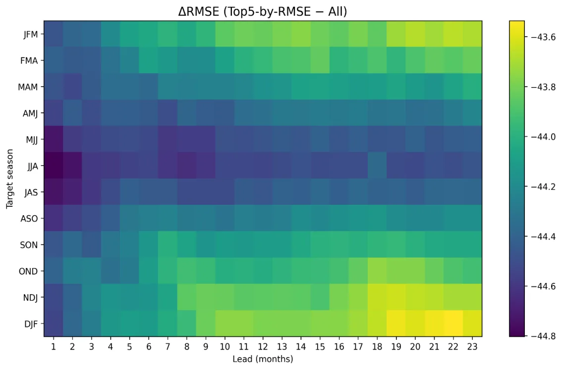
They used an ensemble of 40 ENSO forecasts generated by a modern high-resolution model. Spread among members arises from perturbed initial conditions, stochastic processes, and small changes in parameterizations. Forecasts were verified against the Niño-3.4 index, the average sea surface temperature anomaly in the region 5°S–5°N, 170°W–120°W. Observational data came from the ERSST dataset. For each pair of lead time and target season, members were ranked by two metrics: RMSE (root mean square error, reflecting amplitude accuracy) and Pearson correlation (reflecting phase agreement). Then the top five by each metric were selected, combined with weights proportional to their presence in both lists, and compared with the equally weighted average of all 40 members.
Results
The selected subgroup consistently outperforms the full ensemble on both metrics at all leads from 1 to 23 months. At short leads, the gain is modest: correlation increases by +0.02, and error drops by 0.14 °C. By month 23, the gap becomes dramatic: correlation rises by +0.43 (a 172% increase), and error falls by 0.18 °C (22.5%). The largest improvements occur in the transition seasons SON (September–November) and DJF (December–February), when accurately predicting the onset and maturity of an event matters most. Error reduction is especially strong in mid-year seasons JJA (June–August) and MJJ (May–July). Statistical tests confirm that at leads beyond 12 months, more than 85% of lead–season pairs show significant correlation improvement, and nearly 80% show significant error reduction.
Implications
This work proves that existing ensembles hide a reservoir of accuracy that can be tapped by simple member selection. Unlike neighboring studies that build new neural or hybrid predictors, here neither the model nor the computational cost changes, only the way existing forecasts are combined. This is the first rigorous quantitative estimate of how much can be gained by selecting members specifically for long-lead ENSO forecasting across all seasons and leads.
Future development
The next step is to learn how to identify strong members in real time, when future observations are not yet known. This requires reliable methods for estimating forecast error without access to verification, as well as adaptive schemes that update member weights as new data arrive. If such tools can be built, the retrospective gain could become an operational advantage for forecasting centers.
Impact
The method could be transferred to forecasting other climate phenomena, such as the Indian Ocean Dipole or the North Atlantic Oscillation. It is also applicable to multimodel ensembles, where the members are whole models.
Next steps
Develop procedures for real-time forecast error estimation and test them on historical data. Then check whether the gain persists when moving to multimodel ensembles and under different climate change scenarios.
Key open problems
This work directly addresses the 'spring predictability barrier', the sharp drop in ENSO forecast skill when crossing spring. It shows that selecting ensemble members can soften this barrier and extend the useful forecast horizon to two years, which remains one of the main unsolved problems in climate predictability.
The knowledge machine's view
This section is addressed to the author of the paper and their colleagues. Neighbouring works were found by meaning-based search across our archive, not by word overlap. We do not review: we show the field around the work.
What the work does
The authors used an ensemble of 40 ENSO forecasts, ranked the members by RMSE and correlation for each lead–season pair, selected the top five by each metric, and combined them with weights. Comparison with the equally weighted mean showed an increase in correlation up to +0.43 and a reduction in error to 0.18 °C at a 23-month lead, especially in transition seasons.
Where its strength is
The study shows that simply selecting ensemble members without modifying the models yields a substantial gain in long-lead ENSO forecast accuracy, particularly beyond one year, where traditional methods are weak.
Where it could go next
- It might be interesting to see how the member selection method combines with hybrid statistical–dynamical approaches that account for cyclic components of predictability.based on: A Forecast That Remembers the Cycle arXiv:2602.18949
- A related study improves forecasts by accounting for seasonal predictability; adapting selection to specific seasons might yield additional gains.based on: Space Weather by the Seasons arXiv:2605.27057
- Our archive includes an example of using neural networks for ENSO forecasting; combining selection with training on selected members could open new possibilities.based on: El Niño Can Be Predicted a Year and a Half in Advance arXiv:2601.12251
Worth trying
- Test whether the selection benefit persists when using other metrics, such as rank correlation or error during specific ENSO phases.
- Investigate how the composition of the best members changes from year to year and whether their emergence can be predicted in advance.
- Apply selection not to individual members but to clusters of forecasts to reduce noise from individual outliers.
Why this may matter
If selection consistently improves forecasts at leads longer than a year, it could enhance the practical value of long-lead El Niño warnings for agriculture, energy, and risk management.
Nearby works in our archive
- El Niño Can Be Predicted a Year and a Half in Advancesimilarity 0.56
- Space Weather by the Seasonssimilarity 0.53
- Weather forecast on a single GPUsimilarity 0.50
- Solar Cycles: How Magnetic Swings Sway the Futuresimilarity 0.48
- A Forecast That Remembers the Cyclesimilarity 0.48
- Solar Flares: Forecasting with Confidencesimilarity 0.47
The archive is sparse around this work: the closest review is only 0.56, against a usual 0.64. It looks like few have drilled nearby.
At a 23-month lead, the selected five members achieve a correlation 0.43 higher than the ensemble average, as if the forecast became almost one and a half times more 'in sync' with reality. And the computational cost does not increase by a single ruble.
Key numbers
- correlation gain at 23 months: +0.43
- RMSE reduction at 23 months: 0.18 °C
- number of ensemble members: 40
- maximum forecast lead: 23 months
- fraction of significant improvements at long leads: >85%