least squares fitting

A translator at the negotiating table doesn't listen to every word; they grasp the meaning of whole phrases. Electron microscopy poses a similar challenge: you need to figure out the crystal's thickness and its tilt in the beam, and all you have is a diffraction pattern, a mosaic of thousands of bright and dark spots.

Two photographers shoot the same mountain. One takes a hundred shots from the summit and only a couple from the base; the other does the opposite. If you try to align their images, the algorithm might decide that the summit in one photo matches the summit in the other simply because there are many similar points there, not because it's the same spot. Sampling density throws it off.

A camera looks at two distant sparks. They're so close together that they merge into a single fuzzy blob. It seems impossible to tell them apart — the classic limit of optical microscopy has been reached. But quantum mechanics hints that the light field still holds a secret about where each spark sits.

You could send a short radio pulse toward a black hole and wait for the reflected echo. Intuitively, the shorter the signal, the better it would probe the finest details of spacetime right at the horizon: that region from which even light cannot return.

4 610 universes — that's exactly how many cosmological models astrophysicists needed to show that the familiar Gaussian mask no longer works for next-generation data. Future sky surveys, such as the Euclid mission and the Vera C.

Gravity isn't just the force that keeps us on the floor. On cosmic scales, it conducts galaxies, bends light rays, and decides the fate of everything. A century ago, Einstein described it as the curvature of space and time.

Reconstructing a full picture from fragments is like discerning an orchestra's melody in a noisy hall. Such challenges arise in photometry, where a star's brightness is recovered from faint twinkling. Traditional methods need precise noise information, which is almost always unknown.

The standard approach to a certain class of machine learning problems is like a spring that's been stretched and then forgotten: standard methods artificially inflate the problem's size, turning computations into a black hole for memory and time.

A laser is like a tuning fork that rings at a single note. But even in complete silence, its sound trembles slightly. Previously, it was thought that this tremor, random kicks from spontaneous emission of light by atoms inside the laser, was the main limit to precision.

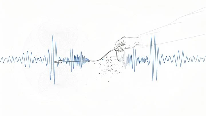
Statistical models are an attempt to stretch a perfect mathematical web over the uneven landscape of data. When a model resists, it emits tension, but we've grown accustomed to ignoring it. Researchers spend hours staring at residual plots, trying to guess where the model is 'coming apart at the seams.' Squealer translates this resistance into sound.

Ordinary neural networks learn from examples, like a person memorizing tunes by ear. But networks with physical laws embedded from the start resemble a musician who knows notes and harmony: they can play a new piece from just a few chords. Instead of mindless memorization, they use equations like energy conservation or motion.

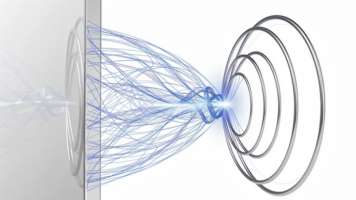
Light needs space. A camera lens sits several centimeters from the sensor so the rays have room to focus. Now, that gap has been squeezed to the thickness of a sheet of paper, and light still behaves as if it had traveled its rightful centimeters. That's what 'spaceplates' do: flat elements that mimic free-space propagation.

In a big city after rain, water collects in the same low spots no matter where the first drops fall. An hour later, the pattern of puddles hardly depends on where the downpour started. That is equilibrium — the outcome a system reaches regardless of its start, once the details are forgotten.

A laser flash lasts a few femtoseconds — imagine a single instant stretched into a million parts. Such a flash mixes many colors, from red to violet. Instruments that measure the pulse shape often err: they see some colors well and others poorly, blurring the picture. The authors propose a simple fix.

A dense social network: everyone is connected to almost everyone else, and in this web it's hard to see who really matters. Too many threads — computers choke, simulations stall. Scientists have figured out how to prune such networks without losing what's essential. The idea is to remove connections that don't participate in shortest paths.

A microbe with flagella rows through water the way a person rows with their arms. But if a person swims breaststroke, they go forward, while a microbe goes in a spiral. The reason is that a microbe has no single direction: each part of its surface pushes water in its own direction, and the body twists like a corkscrew.

Glowing spots on a dark background: that's what single-molecule images from MINFLUX look like. This microscope can reveal details smaller than five nanometers: roughly ten thousand times thinner than a human hair.

Dark matter makes up 85% of the matter in the Universe, yet remains invisible. It only reveals itself through gravity. We can catch it by its cosmic 'hum' — a faint vibration that permeates space. A single detector is powerless here: the signal is too quiet. Physicists turn many sensors into a quantum ensemble.

In the silent heart of creation, where particles converge and part, an act of pure harmony is born. Two Higgs bosons meet and for a fleeting moment form a single whole — and if one demands that their quantum entanglement always reaches its limit, like a tuning fork setting a perfect pitch, then the equations suddenly light up with a new symmetry.

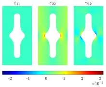
A mechanical testing lab is like a kitchen where a chef tastes a dish to guess the recipe. For an anisotropic material, one that is stiffer along its fibers than across them, a single taste is not enough. You need three or more separate tests, each with its own specimen. Engineers have spent years refining specimen shapes by hand, relying on intuition and experience.

An optician turns the frame, adjusts the focus, and a blurry spot becomes a sharp image. The new algorithm GOAL works much the same way: it rotates the data cloud, compresses redundant dimensions, and brings into focus what truly matters.

Imagine a border river that separates two countries. On one bank live one group of people, on the other, another. The boundary between them is not always obvious: in some places the river is wide and calm, in others narrow and turbulent. But it is exactly where the current changes abruptly that the border becomes most noticeable.