Bayesian inference

In a rubber band stretched in the lab, three different elasticity mechanisms operate simultaneously. At small strains, Hooke's law prevails; at intermediate strains, entropic chain elasticity; at large strains, strain-induced crystallization.

A photographer shoots the same landscape with three different lenses. Every shot shows the same scene, but the softness of detail, the sharpness of edges, and even how visible small objects are all shift from one lens to the next. Brain maps work the same way: the same dataset, run through different smoothing filters, tells slightly different stories about aging.

An interpreter gets distracted by every rustle in the hall, and a one-hour meeting stretches into two. Similarly, molecular foundation models learn the language of molecules from vast corpora, but each new conversation requires fine-tuning. Monroe changes the rules: it doesn't learn a new language but instantly finds common meaning from a few examples.

A protein engineer is like a chef trying to make a dish that is tasty, healthy, and cheap all at once. Change one ingredient, and you risk ruining another. In the past, computer assistants could only evaluate protein properties one at a time, missing how they are connected.

When two heavy nuclei smash into each other at enormous speeds, they don't collide as whole objects like billiard balls. Only part of their matter comes into contact. How many nucleons (protons and neutrons) actually took part in the collision, and how many flew past, is not known in advance. All subsequent measurements depend on this number, but it cannot be observed directly.

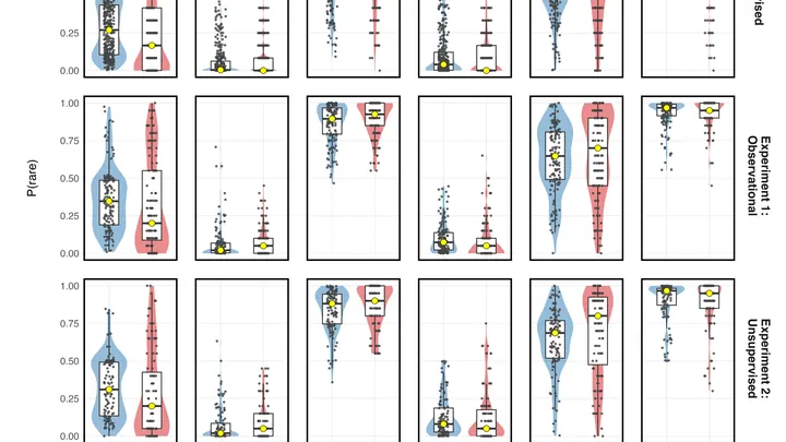
In a warehouse, there are boxes of apples and pears. There are many apples and few pears. But when the stock clerk says "a fruit with smooth skin," we are somehow more likely to recall the rare pear than the common apple. This is the inverse base-rate effect — a persistent glitch in how the brain resolves ambiguity between categories.

A cosmic "caliper" will soon measure a neutron star to within a hundred meters. For an object a couple dozen kilometers across, that's like measuring the thickness of a human hair from a kilometer away. A neutron star is the remnant of an exploded supernova.

A Dictyostelium amoeba crawls across glass. Its path is recorded — a chain of points on a plane. But what forces are pushing it? Inside the cell, a molecular motor works: proteins pull, the membrane springs, water presses.

Two hundred million stars. In the heart of the Galaxy, where the future survey by the Nancy Grace Roman telescope will aim, about 250 times during its mission the light of one of them will flicker at an invisible touch.

4 610 universes — that's exactly how many cosmological models astrophysicists needed to show that the familiar Gaussian mask no longer works for next-generation data. Future sky surveys, such as the Euclid mission and the Vera C.

Reconstructing a full picture from fragments is like discerning an orchestra's melody in a noisy hall. Such challenges arise in photometry, where a star's brightness is recovered from faint twinkling. Traditional methods need precise noise information, which is almost always unknown.

Automatic speech judges are algorithms that evaluate pronunciation and emotions. However, they often work like a food critic who delivers a verdict after reading the menu but not tasting the dish.

Look into the night sky — before you is not a scattering of lights, but a multi-layered manuscript. Under the bright ink of stars and galaxies appears a faded, almost erased text.

On a topographic map, raindrops choose their path: falling on one slope, they flow into River A; on the other, into River B. An observer sees only the winding rivers (the response variables Y) and knows which slope the water came from (the instrument Z), but cannot see the drops themselves (the unobserved factors ε).

The Universe is not silent: it is filled with a continuous gravitational-wave hum. In a decade, the LISA space observatory will tune its "ears" to the millihertz range, and the richest source will be our Galaxy — tens of thousands of white dwarf pairs whirling in a frantic dance.

We're used to thinking that noticing only confirmations of our guesses is a mistake. But recent calculations, inspired by wave behavior, flip that view. It turns out that the habit of seeking the familiar is the best way to reduce information noise (scientists call it entropy).

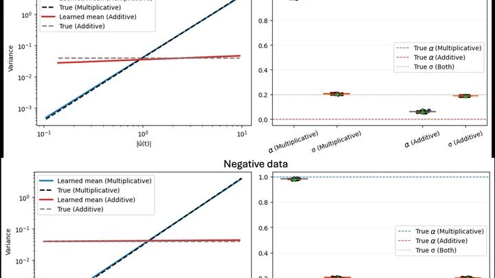
Population growth from a distance looks like a train picking up speed: it crawls at first, then gains momentum. But look closely at the data, and the picture blurs. One measurement shows a dozen individuals, another a hundred. Classical models wipe away this scatter like annoying smudges on a lens. They assume the noise is uniform and simply ignore it.

You buy a new kitchen scale, but instead of exact weight, it only shows deviations from some "norm." To find out how much an apple weighs, you first have to weigh dozens of other apples and calculate the average.

A lab sends a robot a list of a thousand candidate molecules for a new drug. The predictor robot, trained on old data, gives each one a 'fit or no fit' score. But when the list comes from an unfamiliar area, a different virus or a rare tumor, the robot starts to get confused. Its confidence stays high, while actual hits drop to zero.

A spectrum is like a photograph of a material's inner workings, taken with light. When a beam passes through or reflects off a sample, molecules leave characteristic dark bands, peaks, on that photograph. But if the image is overexposed or veiled in gray, making out details becomes nearly impossible.

Dip your finger into water once, and from that single sensation, try to guess its temperature. In the quantum world, such one-shot measurements happen all the time, except you have to guess invisible parameters: say, the squeezing strength of a laser beam.

The hunt for life on distant planets is like diagnosing a rare disease with a test of unknown accuracy. A single positive result means nothing: maybe it's a glitch? We search the atmospheres of exoplanets (worlds around other stars) for traces of water and other compounds, but any signal could be a false alarm.

Your hand rests on the table, and two short vibrations arrive at your wrist — one after the other. You need to say which is stronger. The task seems simple, but the answer depends on which vibration came first. If the first is weak and the second is strong, the difference feels larger than when they are swapped.

An album with hundreds of family photos holds countless stories. If you look at each picture on its own, you might easily decide that Uncle is a real giant: that day he happened to stand a step higher than everyone else. But flip through the whole album, and it becomes clear — his height is perfectly ordinary; it's just that a step showed up in a couple of frames.

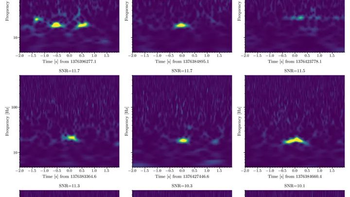
In the headphones used to listen to a distant orchestra, there is an occasional crackle. The crackle can be so loud that it drowns out the music or even blends in with it.

When a neutron or proton enters an atomic nucleus, it behaves like a ball hitting a rough wall: it can bounce off in different ways, depending on where it hits.

A chef's knife and a peeler each handle different tasks, but when a cook learns a new recipe, they often grab the same knife for everything. The brain seems to do the same when mastering a new skill of distinguishing patterns. In the experiment, monkeys trained for weeks to tell apart barely noticeable differences in complex patterns.

Light born at the moment of the Big Bang has traveled to us for almost 14 billion years. But along the way, it passed through the gravitational fields of galaxies and clumps of dark matter, which bent its rays. To an observer, this looks like an image stretched and smudged by an old window pane.

To understand a mechanism, you have to poke it. A child taking apart an alarm clock doesn't just stare at the gears: they turn the wheel and listen to how the ticking changes. Scientists do the same: instead of passive observation, they feed specially chosen signals into the system and watch the response.

Stars on the outskirts of galaxies rotate faster than predicted by the laws of physics if only visible matter is considered. This paradox was uncovered in the 20th century by Vera Rubin and Fritz Zwicky.

Old weather records hold surprises: the thermometer suddenly jumps by half a degree, not because of the weather, but because the station switched instruments. Such abrupt shifts in data are called changepoints, and separating them from genuine climate signals is a challenge statisticians grapple with.

Genetic diagnostics is like comparing two photos taken with different cameras. If one camera slightly shifts the colors, the image will show "defects" that don't exist in reality.

A neutron star is a sphere the size of a city, but it weighs as much as one and a half Suns. Inside such a sphere, matter is so compressed that a teaspoon of it would weigh billions of tons. But physicists don't fully know what this matter is made of.

Inside a neutron star, matter is compressed to unimaginable densities. Previously, scientists speculated about its exact makeup, cycling through possible equations linking pressure and density. The new method tosses out guesswork: it directly ties the measurable mass and radius to the internal structure.

The galaxy is like a city at night: most windows shine steadily, but sometimes a skyscraper lights up all its lights and then goes dark. Just like that, according to a new hypothesis about planets around alien stars (exoplanet), we might first notice another civilization — by a short but blinding flash that could mark its demise.

A rough sketch of a portrait: a few confident lines define the shape, but the details are not yet refined. That is how a parametric model, such as vector autoregression (VAR), describes a time series: it captures the main structure, but if the real data deviate from its assumptions, the portrait comes out distorted.

A meteorologist stares at a pressure map, trying to figure out where the cyclone will go. They have a model, but it is flawed, and fresh measurements, but they are incomplete. Merging the two so that the forecast remains physically meaningful is harder than it seems: classical methods sometimes produce negative temperatures or impossible probabilities.

An interpreter at an important negotiation keeps a draft of their speech at hand but checks against the live conversation as they go: if what is said diverges from the prepared text, they adjust the translation on the fly.

A translator who jumps at every rustle in the hall starts mixing up words by the end of the meeting. Their confidence in being right grows, while their accuracy drops. That is roughly how poorly calibrated probabilistic forecasts behave: the model claims a high probability for an event, but reality disagrees.

The barometer in the port of Papeete on Tahiti and the one in Darwin, Australia, are separated by 7,400 kilometers. When one shows high pressure, the other often shows low, and this difference, called the Southern Oscillation, drives rainfall from India to Brazil. Predicting it even a month ahead is a problem with a century-long history.