Geometric phase control is a technique for manipulating quantum states by exploiting the geometric phase—a phase acquired by a quantum system that depends only on the path taken through its state space, not on the speed or duration of the journey. Unlike dynamic phases, which arise from energy differences and are sensitive to timing and noise, geometric phases are inherently robust, making them valuable for precise quantum operations. This approach is central to fault-tolerant quantum computing and quantum communication, where maintaining coherence is critical.
History
The geometric phase was formalized by Michael Berry in 1984, building on earlier work by Pancharatnam (1956) and Aharonov and Bohm (1959). The idea of using it for quantum computation was proposed in the late 1990s.
How it works
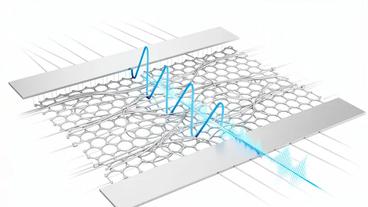
When a quantum system evolves along a closed loop in its parameter space, it returns to its original state but with an extra phase factor—the geometric (Berry) phase. By carefully designing electromagnetic field pulses to guide the system along specific loops, researchers can control this phase to implement quantum gates. Because the phase depends only on the loop's geometry, it is immune to certain types of errors, such as fluctuations in pulse timing or field strength.
The geometric phase is so robust that it appears in classical systems too—for example, in the swing of a pendulum on a rotating platform, where the direction of swing shifts after a full rotation.
A navigator with a paper chart plots the route before setting sail. If the ocean changes—the current shifts, the wind picks up—the chart stays the same. The ship follows an outdated path, and the crew has to correct the course by hand.
Imagine a ladder whose rungs are tiny magnets. If neighboring magnets point in opposite directions, the ladder is "calm." But if you make them all point the same way, the whole structure becomes magnetized and "stubborn."
Scientists built such a ladder from germanium atoms — a semiconductor used to make transistors.
In an ultracold cloud of atoms cooled to near absolute zero, regions with different spin orientations emerge, like patches with different magnetization. The boundaries between them are called domain walls. Usually they are stationary, but in this experiment the walls started moving on their own.
In a pot of boiling water, steam bubbles appear and disappear — a similar struggle takes place in two-dimensional materials. Here, electrons both create magnetism and try to extinguish it.
A cup of hot coffee sometimes freezes faster than cold tap water. This paradox, known as the Mpemba effect, has long been considered a curiosity of classical physics. Now its quantum counterpart has helped test and tune quantum processors — devices that may one day power supercomputers.
The quantum world is tricky: sometimes particles confined to a flat layer and pierced by a strong magnetic field start behaving like a liquid made not of whole electrons but of their fractions — fractional charges. This is the fractional quantum Hall effect.
Hot tea cools down, and ice cream melts — heat always flows from warm to cold, and this law seemed unbreakable. But in the quantum world, even familiar rules can be rewritten. Physicists placed a tiny mechanical resonator (a vibrating bridge the size of a microbe) in an optical cavity between two mirrors.
A delicate watermark on wet paper, and a fogged-up glass before your eyes. That's roughly what reading quantum states of light looks like: fragile photon patterns get distorted by losses, and detectors catch only a small fraction of the signal.
For a long time, identifying quantum phases was like interrogating a witness: you had to reach every corner of the system to uncover its secret. In the era of Landau, order was tied to symmetry breaking and a local parameter — everything plain as day.
Imagine a quantum phase transition as an intricate dance. Electrons whirl in strict order, each step representing their spatial arrangement, and the rhythm their dynamics. For decades, physicists could only see a blur of motion, unable to tell if the figures were changing or the music speeding up.
A quantum computer is like an orchestra where every musician must hit their note exactly. If one plays off-key, the melody falls apart. The musicians here are qubits, storing information.
A magnetic field holds a tiny particle in mid-air, like an invisible dance partner. A special tuning of the field creates a trap with two "positions." In the ordinary world, a dancer occupies only one, but in the quantum world — both at once. Physicists have learned to achieve this for dust grains weighing trillionths of a gram.
In the first moments after the Big Bang, the Universe was like a supercooled bottle of champagne. In addition to ordinary matter, it concealed a dark sector — an invisible sparkling “wine” of fields and particles, candidates for dark matter.
A black hole is not a dead object. After a disturbance, such as merging with another hole, it rings like a bell. This ring is not just a sound but a complex set of damped oscillations called quasinormal modes. Their frequency and damping rate depend on the hole itself: its mass, charge, and spin.
In a long corridor, a crowd of people tries to keep as far apart as possible. In a spacious hall, they would simply spread out, but here the walls squeeze them so tightly that they have to move single file, coordinating every step. Electrons in graphene layers twisted by a tiny angle behave in a similar way.
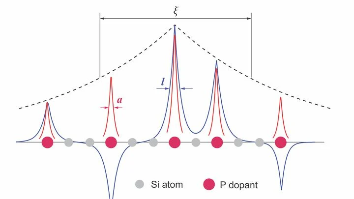
Toss a handful of phosphorus into silicon, and at a certain impurity concentration the material suddenly starts conducting electricity. This is a metal-insulator phase transition, and it happens abruptly. But what exactly changes in the electron wave functions when an insulator becomes a metal?
Gravitational-wave observatories are like a keen ear listening for distant rumbles of cosmic catastrophes. To catch the faint whisper of merging black holes, detectors of gravitational waves use specially prepared light — known as squeezed vacuum.
In the world of atoms and particles, everything tends toward rest: particles lose energy, just as a swing slows down due to energy loss (friction). But many devices — from hydrogen masers to atomic clocks — live by repetitive cycles.
An ordinary magnet is like a compass: its needle points north. But a quantum compass can look in both directions at once. If a magnet floating in a vacuum is gently spun, its electron 'tops' synchronize so the whole piece of metal starts living by the rules of the microworld — freezes in a superposition, like a split pointer.
A quantum computer measures a molecule's energy much like an old tape measure that only has markings every meter. If the actual length of a table is 2.37 meters, the tape shows “two and a bit,” and you can't do better. Physicists call this resolution: the step of the grid, finer than which you cannot go.
The authors of the new work turn this flaw into an advantage.
A soap bubble hangs in the air, and its shape already contains everything needed to calculate the internal tension. A similar principle worked in a new study on quantum gravity. Physicists took a closed surface, an analog of such a bubble, and specified a few numbers on it: for example, the electric field strength and the curvature.
A person hunting for keys mentally runs through places where they might be. A bird that tucked hundreds of seeds into crevices in autumn retrieves them flawlessly in winter. How can a brain hold so many addresses when all birds have roughly the same number of neurons? The answer lies in geometry.
A quantum computer is like an orchestra where each musician plays their part, but if one hits a wrong note, the melody falls apart. Errors arise constantly: from thermal jitter, from imperfect instruments. To keep the symphony going, you need a "conductor" who hears the off-key notes and corrects them on the fly.
The birth of the universe is often compared to inflating a balloon: in the first moments, it stretched rapidly. But the very "rubber" of this balloon was probably not perfectly smooth — rather, it was covered with the finest ripples.
When you flip a switch, the light doesn't come on immediately — electrons in the wires need time to 'get going' and move together. In ordinary metals and semiconductors, current builds up gradually, like water in a hose when you first open the tap.
A laser beam hits an atom, and an electron is knocked loose. It accelerates, returns, and, crashing into the atom, emits a flash of light — a harmonic. If there are two light beams and they are crossed like an intersection, the electron can choose different routes. In the new experiment, the two beams had comparable strength and were directed at right angles.
Water can be ice, liquid, or steam. Physicists call these states phases. In theory, each phase has its own measure — a way to describe how likely it is. But not every measure you can imagine occurs in nature. Some phases are real, while others are just mathematical illusions.
Scientists have found a simple criterion that separates reality from mirage.
A light pulse can be compared to a musical chord: several notes sound simultaneously, each with its own loudness and phase. In quantum optics, such 'chords' are called multimode squeezed states.
Fireflies flash in a dark forest: you see each flash, but not the flight. A quantum gas microscope can show individual cold atoms, like those fireflies. But until now, it couldn't tell you how fast they're moving.
Now scientists have found a way to fix that.
A gold particle a few nanometers across looks like a tiny faceted diamond, but with five faces instead of the usual ones. Inside it hides a defect, like a crack in glass that can either heal or shatter the whole object. Scientists set out to discover what makes this defect move and disappear.
The quantum world loves order, but reality often brings disorder. In this work, physicists study one-dimensional chains of spins — tiny magnetic arrows that can point up or down. Usually, topological phases (stable states protected by symmetry) are defined for pure states, where each arrow is precisely known.
A quantum dot is like a tiny island where one or a few electrons can settle. In this new work, such an island was connected to two 'seas' of electrons: one flat like a pancake, the other bulky like an ocean. Electrons can hop from the island to the seas and back, and this hop depends on the shape of the electron's wave on the island.
A typical accelerator is like an assembly line where electrons are the workpieces. To get the desired X-ray pulse, the workpiece is fine-tuned after it's already on the line: squeezed, filtered, corrected. In the new work, engineers decided to take a different approach — shaping the workpiece before it even hits the conveyor.
At LCLS-II, electrons are knocked out of a metal by a short laser pulse.
A laser beam holds a single ion in a vacuum, and that ion behaves like a ball trapped between two cups. The cups aren't pits in the ground but regions where the ion energetically prefers to be. In the classical world, a ball would roll into one cup and stay there.
In a small copper box, resembling a matchbox, magnetic waves reside. They arise in a tiny crystal of yttrium iron garnet when radio waves are passed through it. Two waves with different characters (one fast, the other slow) usually ignore each other. But when their frequencies match, a dance begins: the waves either merge into one strong wave or cancel each other into complete silence.
If you shake a box of sand long enough, patterns appear on its surface — patterns that weren't there when the box was still. It's the same here: physicists took a cloud of cold atoms, trapped them in an optical lattice, and began shaking it periodically. This gave rise to a new state in the atoms, like a new pattern in the sand that doesn't exist without the shaking.
You can edit a cell perfectly, and it still turns out useless. The gene is fixed exactly as planned, yet the cell behaves unpredictably: it drifts, changes fate, loses safety. It's like fixing one gear in a watch, but the watch still runs wrong because the whole mechanism is out of sync.
Previously, a cell was viewed as a list of independent parts.
A fingernail-sized piece of ceramic is squeezed in a vise, and its internal structure rearranges like clay under your fingers. Inside, orderly rows of tiny domains line up where they were once randomly oriented. After this 'massage,' the crystal lets light through almost like glass and, at the same time, generates a strong electric charge when bent or pressed.
Picture heavy balls resting on a stretchy trampoline: each one sinks into the fabric, and their dents overlap, causing the balls to roll toward each other. This analogy helps explain how gravity — the curvature of spacetime — links massive particles. But what if you bring gravity and quantum mechanics together?